1. Decision Theoretic Planning

2. Overview Decision processes and Markov Decision Processes (MDP)
Rewards and Optimal Policies
Defining features of Markov Decision Process
Solving MDPs
Value Iteration
Policy Iteration
POMDPs

3. Rewiew: Decisions Under Uncertainty
Some areas of AI (e.g., planning) focus on decision making in domains where the environment is understood with certainty
Here we focus on an agent that needs to make decisions in a domain that involves uncertainty
An agent’s decision will depend on:
what actions are available. They often don’t have deterministic outcome
what beliefs the agent has over the world
the agent’s goals and preferences

4. Decision Processes
We focus on situations that involve sequences of decisions
The agent decides which action to perform
The new state of the world depends probabilistically upon the previous state as well as the action performed
The agent receives rewards or punishments at various points in the process
The agent’s utility depends upon the final state reached, and the sequence of actions taken to get there
Aim: maximize the reward received

5. Markov Decision Processes (MDP)
For an MDP you specify:
set S of states, set A of actions
Initial state s0
the process’ dynamics (or transition model)
P(s'|s,a)
The reward function
R(s, a,, s’)
describing the reward that the agent receives when it performs action a in state s and ends up in state s’
We will use R(s) when the reward depends only on the state s and not on how the agent got there

6. Planning Horizons
The planning horizon defines the timing for decision making
Indefinite horizons: the decision process ends but it is unknown when
In the previous example, the process ends when the agent enters one of the two terminal (absorbing) states
Infinite horizons: the process never halts
e.g. if we change the previous example so that, when the agent enters one of the terminal states, it is flung back to one of the two left corners of the grid
Finite horizons: the process must end at a specific time N
We focus on MDPs with infinite and indefinite horizons

7. Information Availability
What information is available when the agent decides what to do?
Fully-observable MDP (FOMDP):
the agent gets to observe current state st when deciding on action at .
Partially-observable MDP (POMDP)
the agent can’t observe st directly, can only use sensors to get information about the state
Similar to Hidden Markov Models
We will first look at FOMDP (but we will call them simply MDPs)

8. Reward Function
Suppose the agent goes through states s1, s2,...,sk and receives rewards r1, r2,...,rk
We will look at discounted reward to define the reward for this sequence, i.e. its utility for the agent

9. Solving MDPs
In search problems, aim is to find an optimal state sequence
In MDPs, aim is to find an optimal policy π(s)
A policy π(s) specifies what the agent should do for each state s
Because of the stochastic nature of the environment, a policy can generate a set of environment histories (sequences of states) with different probabilities
Optimal policy maximizes the expected total reward, where the expectation is take over the set of possible state sequences generated by the policy
Each state sequence associated with that policy has a given amount of total reward
Total reward is a function of the rewards of its individual states (we’ll see how)

10. More formally A stationary policy is a function: Utility of a state
For every state s, л(s) specifies which action should be taken in that state.
Utility of a state
Defined as the expected utility of the state sequences that may follow it
These sequences depend on the policy л being followed, so we define the utility of a state s with respected to л (a.k.a value of л for that state) as
Where Si is the random variable representing the state the agent reaches after executing л for i steps starting from s

11. More Formally (cont.)
An optimal policy is one with maximum expected discounted reward for every state.
A policy л* is optimal if there is no other policy л’ and state s such as
Uп’(s) > Uп*(s)
That is an optimal policy gives the Maximum Expected Utility (MEU)
For a fully-observable MDP with stationary dynamics and rewards with infinite or indefinite horizon, there is always an optimal stationary policy.
END REVIEW

12. Overview Brief review of simpler decision making problems
one-off decisions
sequential decisions
Decision processes and Markov Decision Processes (MDP)
Rewards and Optimal Policies
Defining features of Markov Decision Process
Solving MDPs
Value Iteration
Policy Iteration
POMDPs

13. Value Iteration
Algorithm to find an optimal policy and its value for a MDP
The idea is to find the utilities of states, and use them to select the action with the maximum expected utility for each state

14. Value Iteration: from state utilities to л*
Remember that we defined the utility of a state s as the expected sum of the possible discounted rewards from that point onward
We define U(s) as the utility of state s when the agent follows the optimal policy л* from s onward (i. e., U л*(s))
aka value of л*

15. U(s) and R(s) Note that U(s) and R(s) are quite different quantities
R(s) is the short term reward related to s
U(s) is the expected long term total reward from s onward if following л*
Example: U(s) for the optimal policy we found for the grid problem with R(s non-terminal) = and γ =1

16. Value Iteration: from state utilities to л*
Now the agent can chose the action that implements the MEU principle: maximize the expected utility of the subsequent state
expected value of following policy л* in s’
states reachable
from s by doing a
Probability of getting to s’ from s via a

17. Example
To find the best action in (1,1)

18. Example
To find the best action in (1,1)

19. Example
To find the best action in (1,1)

20. Example To find the best action in (1,1)
Plugging in the numbers from the game state above, give Up as best action

21. Finding Utilities Great, but how do we find the utilities?
Value iteration exploits the relationship between the utility of a state and the utility of its neighbours
So the utility of following the optimal policy in s is
Reward sequences for the states reached by following the optimal action in sk
Immediate reward for s
Expected utility of state s’ reached by action a in s

22. Finding Utilities
Given N states, we can write an equation like the one below for each of them
Each equation contains N unknowns – the U values for the N states
N equations in N variables (Bellman equations)
It can be shown that they have a unique solution: the values for the optimal policy
Unfortunately the N equations are non-linear, because of the max operator
Cannot be easily solved by using techniques from linear algebra
Value Iteration Algorithm
Iterative approach to find the optimal policy and corresponding values

23. Value Iteration: General Idea
Let U(i)(s) be the utility of state s at the ith iteration of the algorithm
Start with arbitrary utilities on each state s: U(0)(s)
Repeat simultaneously for every s until there is “no change”
True “no change” in the values of U(s) from one iteration to the next are guaranteed only if run for infinitely long.
In the limit, this process converges to a unique set of solutions for the Bellman equations
They are the total expected rewards (utilities) for the optimal policy

24. VI algorithm

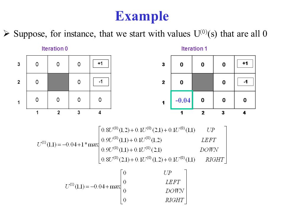
25. Example
Suppose, for instance, that we start with values U(0)(s) that are all 0
Iteration 0
Iteration 1 3 2 1 +1 -1
-0.04

26. Example (cont’d) -0.04 -0.4 Let’s compute U(1)(3,3) 0.76 Iteration 02 1
0.76 +1 -1
-0.04
-0.4

27. Example (cont’d) .76 -0.04 -0.04 Let’s compute U(1)(4,1) Iteration 03 2 1
.76 +1 -1
-0.04
-0.04

28. After a Full Iteration
Iteration 1 3 2 1
-.04
0.76 +1 -1
Only the state one step away from a positive reward (3,3) has gained value, all the others are losing value because of the cost of moving

29. Some steps in the second iteration3 2 1
-.04
0.76 3 2 1
-.04
0.76 +1 +1 -1 -1
-0.08

30. Example (cont’d) -0.08 Let’s compute U(1)(2,3)
Steps two moves away from positive rewards start increasing their value
Iteration 2
Iteration 1
-.04
0.76
0.56 3 2 1
-.04
0.76 +1 +1 -1 -1
-0.08

31. State Utilities as Function of Iteration #
Note that utilities of states at different distances from (4,3) accumulate negative rewards until a path to (4,3) is found

32. Convergence of Value Iteration
Need to define Max Norm:
Defines length of a vector V as the length of its biggest component
If there were two fixed points, they would not get closer together when the contraction is applied to them
When the function is repeatedly applied to any argument, the value must get closer to the fixed point. gets closer to the fixed point, because the fixed point does not move

33. Convergence of Value Iteration
Let U(k+1)represent the utilities of all states at the k+1 iteration of the algorithm.
Be Ut and U(t+1) be successive approximations to the true U*
It can be shown that
So if we view ||U(k) -U*|| as the error in the estimate of U* at iteration k, value iteration reduces it by γ at every iteration
Value iteration converges exponentially fast in number of iterations

34. Convergence of Value Iteration
We can now look at how many iterations N we need to reach an error ε
We saw state utility is bounded by where Rmax is max reward available
Thus, maximum initial error is
Since error is reduced by γ at each iteration, we require

35. Convergence of Value Iteration
Picture shows how N varies with γ for different values of ε/Rmax (c in the figure)
For our sample gridworld

36. Convergence of Value Iteration
Picture shows how N varies with γ for different values of ε/Rmax (c in the figure)
Good news is that N does not depend too much on the ratio
Bad news is that N grows rapidly as γ gets close to 1
We can make γ small, but this effectively means reducing how far ahead the agent plans its actions
short planning horizon can miss the long term effect of the agent actions

37. Convergence of Value Iteration
Alternative way to decide when to stop value iteration
It can be shown that,
The if side of the statement above is often used as a termination condition for value iteration

38. Convergence of Value Iteration
After value iteration generates its estimate U’ of U, one can choose the optimal policy based on a one-step look-ahead from U’
In practice, it occurs that л(final) becomes optimal long before U’ has converged to U

39. Policy Loss For our sample gridworld
Max Error is the maximum error made by the estimated U’ as compared U
|| U’- U||
Policy Loss is maximum difference in total expected value when following л(final) instead of the optimal policy
|| U л(final) - U||

40. Asynchronous Value Iteration
The “basic” version of value iteration applies the Bellman update to all states at every iteration
This is in fact not necessary
On each iteration we can apply the update only to a chosen subset of states
Given certain conditions on the value function used to initialize the process, asynchronous value iteration converges to an optimal policy
Main advantage
one can design heuristics that allow the algorithm to concentrate on states that are likely to belong to the optimal policy
Makes sense: if I have no intention of ever doing research in AI, there is no point in exploring the resulting states
Much faster convergence

41. Storing U(s) vs. Q(s,a)
Value iteration stores the values of U for every state
There is a version of the algorithm that stores for every state and for every action, the expected value of performing that action in that state Q(s,a)
Need to see if
Storing Q(s,a) requires more space because it requires a more values per state
But it is easier and faster to retrieve the actions in the optimal policy

42. Overview Brief review of simpler decision making problems
one-off decisions
sequential decisions
Decision processes and Markov Decision Processes (MDP)
Rewards and Optimal Policies
Defining features of Markov Decision Process
Solving MDPs
Value Iteration
Policy Iteration
POMDPs

43. Policy Iteration
We saw that we can obtain an optimal policy even when the U function returned by value iteration is not optimal yet
Intuitively, if one action is clearly better than all others, the precise utilities of the states involved are not necessary to select it
This is the intuition behind the policy iteration algorithm

44. Policy Iteration Algorithm
πi ← an arbitrary initial policy, U ← A vector of utility values, initially 0
2. Repeat until no change in π
Compute utilities Ui generated by executing πi with current U (policy evaluation)
(b) Compute a new MEU πi+1 using a one-step look-ahead based on Ui (policy improvement)
Watch out, there is no “MAX” here, because the policy is already fixed!
Here there is “MAX” because we need to find out whether there is any other action that does better then the action specified by πi

45. Policy Iteration Policy evaluation: for every s
Once again, we have N equations with N unknown (the current U(s)), but the good news is that they are linear!
The max operator is no longer there because I am not looking for the maximum utility policy, I have picked one already
Can be solved exactly in O(N3) with linear algebra methods

46. Policy Iteration

47. Policy Iteration

48. Policy Iteration

49. Policy Iteration

50. Modify Policy Iteration
O(N3) is good for small state space, but it can be prohibitive if N is large
The good news is that we don’t have to evaluate the policy at every iteration
Do a number of value iteration steps given the current policy л and estimated Uk (simplified value iteration)
This provides a better approximation of U
Then do policy improvement and repeat
Often much more efficient than Value Iteration or Standard Policy Iteration

51. Asynchronous Policy Iteration
Same concept used in Value Iteration
The “basic” version of policy iteration does policy improvement for all states at every iteration
This is in fact not necessary
On each iteration, pick any subset of the states and
apply either policy improvement or simplified value iteration
Given certain conditions on the value function used to initialize the process, asynchronous value iteration converges to an optimal policy

52. Overview Brief review of simpler decision making problems
one-off decisions
sequential decisions
Decision processes and Markov Decision Processes (MDP)
Rewards and Optimal Policies
Defining features of Markov Decision Process
Solving MDPs
Value Iteration
Policy Iteration
POMDPs