Download presentation
Presentation is loading. Please wait.

1
Clusters of galaxies The ICM, mass measurements and statistical measures of clustering

2
Plan of this class The intracluster medium, its origin, dynamics and general properties Evidence of Dark Matter in clusters Masses derived by the virial theorem, x-rays and gravitational lensing Results from studies of gravitational lensing in clusters Statistical measures of clustering

3
The intracluster medium

4
Clusters are among the most luminous X-ray sources in the sky. This X-ray emission comes from hot intracluster gas. X-ray observations provide information on the amount, distribution, temperature and chemical composition of the Intracluster gas

5
For comparison, Cataclismic variables Lx = 10 32 – 10 38 erg/s Milky Way, M31 Lx = 10 39 erg/s Clusters of galaxies Lx = 10 43 – 10 45 erg/s Only Seyferts, QSOs, and other AGN rival clusters in X- ray output Clusters may emit nearly as much energy at X-ray wavelengths as visible L(optical) = 100 L* galaxies = 10 45 erg/s
 = 100 L* galaxies = erg/s")
6
The L x – σ correlation

7
What is the origin of cluster X-ray emission? Answer: hot (10 7 – 10 8 K) low-density (10 -3 cm -3) gas, mostly hydrogen and helium, that fills space between galaxies. At these high temperatures the gas is fully ionized. Two emission mechanisms: 1) Thermal bremsstrahlung (important for T > 4 x 10 7 K) free electrons may be rapidly accelerated by the attractive force of atomic nuclei, resulting in photon emission because the emission is due to Coulomb collisions, X- ray luminosity is a function of gas density and temperature Lx = n electron n ion T 1/2 = rho_gas 2 T_gas 1/2 2) Recombination of electrons with ions (important T < 4 x 10 7 K)
 low-density (10 -3 cm -3) gas, mostly hydrogen and helium, that fills space between galaxies. At these high temperatures the gas is fully ionized. Two emission mechanisms: 1) Thermal bremsstrahlung (important for T > 4 x 10 7 K) free electrons may be rapidly accelerated by the attractive force of atomic nuclei, resulting in photon emission because the emission is due to Coulomb collisions, X- ray luminosity is a function of gas density and temperature Lx = n electron n ion T 1/2 = rho_gas 2 T_gas 1/2 2) Recombination of electrons with ions (important T < 4 x 10 7 K).")
8
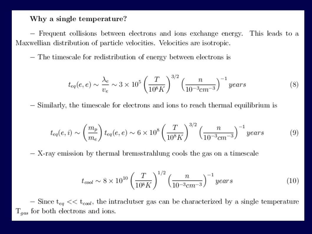
Dynamics of the intracluster gas The intracluster gas can be treated as: An ideal fluid In hydrostatic equilibrium At a uniform temperature

14
X-ray spectra Spectroscopy of the intracluster gas provides information on its temperature and composition Observed spectra show exponential decrease at high- frequencies that is characteristic of bremsstrahlung. Coma Cluster Hughes et al. 93

15
Emission lines due to Fe, Ni and other heavy elements are seen. This suggests that much of the intracluster gas must have been processed through stars. Chemical abundance of the intracluster gas can be measured from the equivalent widths of these emission lines. It is found to be about 30-40% of solar abundance If the galaxies and gas are both in thermal equilibrium in the cluster potential well, then one expects m v(gal) 2 = 3 k b T gas T gas proportional to v(gal) 2
 2 = 3 k b T gas T gas proportional to v(gal) 2.")
16
What is the origin of the intracluster gas? Two possibilities: The intracluster gas once resided in galaxies and was later removed. - this would explain high metallicity of gas - galaxies in the cores of rich clusters are observed to be deficient in HI gas, which suggests that stripping has occurred. The gas is primordial, originating at the time of cluster formation. - but since Mgas >> Mgal it is difficult to understand how so much material could have been stripped from galaxies

17
How much gas is there in clusters?

18
Cluster Mass estimates: X-ray gas

19
The total gas mass in clusters exceeds the total galaxy mass. Gas contributes as much as 10-20% of the total cluster mass. David, Jones and Forman 95

20
Evidence of Dark Matter (DM) in clusters
 in clusters")
21
Dark Matter in Clusters A more accurate name for “clusters of galaxies” would be “clusters of dark matter” Observational evidence suggests that 80-90% of the mass in clusters is in an invisible form 1) What evidence is there for dark matter? 2) How much dark matter is there? 3) What is the distribution within clusters?
 How much dark matter is there. 3) What is the distribution within clusters .")
22
Evidence of Dark Matter in clusters Virial mass estimates If a cluster is in virial equilibrium then its mass can be estimated from M virial = R /G Observations indicate that the total cluster mass exceeds the combined masses of all galaxies by factors of 10-20. Example: the Coma Cluster M virial = 1 x 10 15 h -1 solar masses L tot = 4 x 10 12 h -2 solar luminosities Assuming a typical galaxy with M/L = 10 Then M virial /M galaxies = 25

23
Typical mass to light ratios Globular clusters 1-2 M/L Elliptical galaxies 5-10 h M/L Groups of galaxies 100-300 h M/L Rich clusters 300-500 h M/L

24
Mass to light ratio of Coma

25
Galaxy Dynamics Mass estimate using the Virial theorem

26
X-ray mass estimates If the intracluster gas is in hydrostatic euilibrium in the cluster potential, then the cluster mass can be determined from

27
Gravitational lensing studies provide another independent evidence for DM in clusters

28
Gravitational Lensing – some history 1913 – Einstein predicted that the gravitational field of massive objects can deflect light rays. 1919 – Eddington measured the deflection of starlight by the Sun, confirming Einstein’s prediction. 1937 – Zwicky suggested that galaxy clusters may produce observable lensing. 1987 – First evidence of “strong” gravitational lensing by clusters was found (Lynds/Petrosian, Soucail et al.) 1990 – “Weak” gravitational lensing by clusters was discovered (Tyson et a. 1990). Today – Evidence of lensing has been found for several dozen clusters. New examples are being discovered all the time.
 1990 – Weak gravitational lensing by clusters was discovered (Tyson et a. 1990). Today – Evidence of lensing has been found for several dozen clusters. New examples are being discovered all the time..")
30
1986 – Lynds & Petrossian discover the first gravitational arcs in clusters of galaxies 1987 – Soucail et al. determine the distance to the arc: twice the distance to the cluster that “contains” it. STRONG LENSING

31
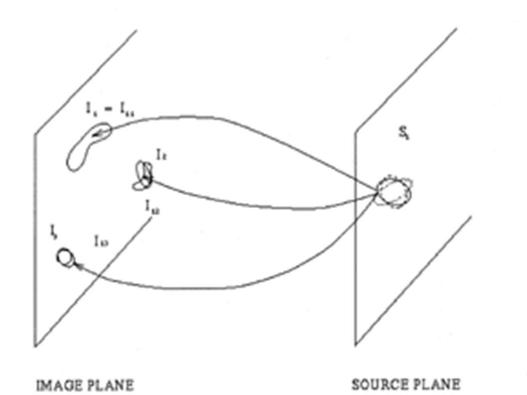
Gravitational lensing: the basic ideas

33
Galaxy cluster Background galaxy Observer Strong lens Weak lens

34
“Strong” lensing occurs when Long arcs and multiple images are produced. “Weak” lensing occurs when Small arclets and distortions are produced.

37
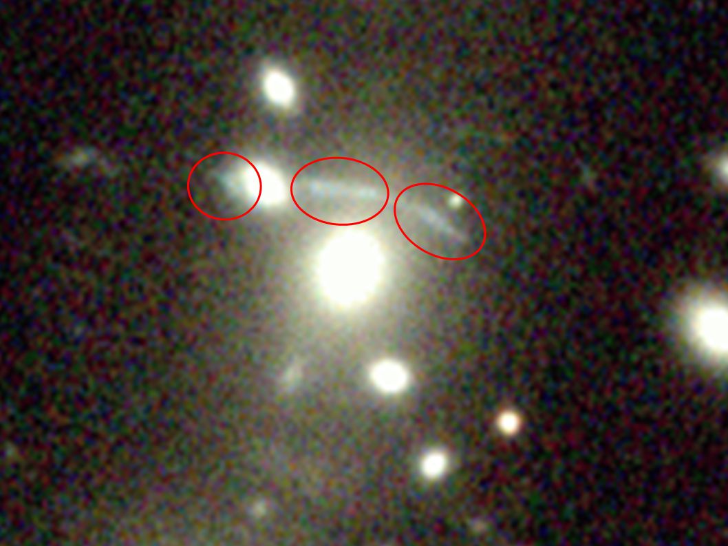
A 1451 z = 0,199 Strong Lensing

39
A 1451 z = 0,199

40
Weak Gravitational Lensing Mellier 99

41
Why Weak Lensing ? Allows the reconstruction of the surface mass density Classical techniques (dynamics of the galaxies and X-ray emission of the hot intra-cluster gas) are based of the assumption of dynamical equilibrium
 are based of the assumption of dynamical equilibrium.")
42
Measuring Faint Galaxy Shapes Cypriano et al. 2005

43
Mass Light Mass Light A2029 In 77% of the cases the center of light and mass distributions are consistent with each other...

44
Mass Light...but there are exceptions MassLight A3739

45
Mass Light Mass Light A4010

46
Mass Light There is a strong alignment between the BGC and the dark mater main axis

47
Comparison with X-Rays T X ~ T SIS,SIE A2744 A1451 A2163

48
Comparison with the Velocity Dispertion A1451 A2744 A2163 σ v ~ σ SIS,SIE

49
The dynamical state of the clusters Most of the clusters appears to be relaxed (lensing dynamical methods) Cluster with T X > 8 keV (σ v >1120 km/s) shows signs of dynamical activity
 Cluster with T X > 8 keV (σ v >1120 km/s) shows signs of dynamical activity")
50
The dynamical state of the clusters A2744 – Virial mass> Lensing > X-rays Girardi & Mezzetti (2001) σ total = 1777 km/s σ A = 1121 km/s σ B = 682 km/s Interpretation: There are two structures along the line of sight Chandra observations confirms fusion along the line of sight (Kempner & David 2004)
 σ total = 1777 km/s σ A = 1121 km/s σ B = 682 km/s Interpretation: There are two structures along the line of sight Chandra observations confirms fusion along the line of sight (Kempner & David 2004)")
51
Which method is the best one ? Weak Lensing Independent of the dynamical state Needs good seeing Reconstruct the 2-D potencial Cannot separate components along the line of sight.

52
Which method is the best one ? X-Rays All Sky Surveys (e.g. ROSAT) can provide large and homogeneous samples Depend of thermal/dynamical state of the ICM Cannot separate components along the line of sight.
 can provide large and homogeneous samples Depend of thermal/dynamical state of the ICM Cannot separate components along the line of sight..")
53
Which method is the best one ? Dynamics of galaxies Depend on the dynamical state of the cluster galaxies (galaxies relaxes later than the ICM) Can separate structures along the line of sight Reliable results depends on a large number of galaxy velocities over a large area (e.g. Czoske et al. 2002) No single method is perfect !
 Can separate structures along the line of sight Reliable results depends on a large number of galaxy velocities over a large area (e.g. Czoske et al. 2002) No single method is perfect !.")
54
What can we learn from gravitational lensing? Gravitational lensing can be used to determine the amount and distribution of dark matter in clusters. Unlike virial or X-ray mass determinations, lensing requires no assumptions about the dynamical state of the cluster! The arc thickness is related to the cluster mass distribution. More concentrated mass distributions produce thinner arcs. Modelling the positions and shapes of arcs and arclets allows the cluster potential to be mapped. Lensing models have become so good that in can predict the locations of faint additional arcs. Gravitational lensing causes images to be magnified. Clusters of galaxies can be used as natural “telescopes”to study extremely distant galaxies that would be otherwise too faint to see. Lensing can also be used to place cosmological constraints, because distances (Dos, Dol, Dls) depend on omega, Ho and lambda.
 depend on omega, Ho and lambda..")
55
z = 5.6 Ellis, Santos, Kneib & Kuijken (2001)
")
56
What have we learned so far from gravitational lensing? Samples of strong and weak gravitational lensing have been found in several dozen clusters. Lensing mass estimates indicate large quantities of dark matter in clusters Lensing mass estimates agree with virial and X-ray masses (with a few exceptions). The exceptions are probably clusters which are not in equilibrium. Hot clusters tend to present dynamical activity (major concern for experiments designed to constrain cosmological parameters). Mass follows light in most cases. Cluster dark matter has a very steep radial distribution. Models of the cluster potential provide strong evidence of substructure in the dark matter distribution. Gravitational lensing has been seen in clusters at z>1
. The exceptions are probably clusters which are not in equilibrium. Hot clusters tend to present dynamical activity (major concern for experiments designed to constrain cosmological parameters). Mass follows light in most cases. Cluster dark matter has a very steep radial distribution. Models of the cluster potential provide strong evidence of substructure in the dark matter distribution. Gravitational lensing has been seen in clusters at z>1.")
57
Clusters as Tracers of Large- scale Structure

58
Why use clusters to map the large-scale structure of the universe? Advantages Clusters provide an efficient way of surveying a large volume of space Cluster distribution provides information about conditions in the early universe Clusters can be seen at great distances Disadvantages Their low space density makes clusters sparse tracers of the large scale structure Results may depend on the chosen cluster sample Redshifts of many clusters are still unmeasured

59
Velocidade

60
De Lapparent et al. 1988 Velocidade d=v/Ho Lei de Hubble The Cfa Slice

61
Velocidade The Cfa Slice

62
Velocidade The Cfa Slice

63
Large scale structure – 2dF

64
Some history 1933 – Shapley noticed several binary and triple systems among the 25 clusters that he catalogued “it is possible that clusters are but nuclei or concentrations in a very extensive canopy of galaxies”. 1954 – Shane and Wirtanen’s galaxy maps showed “a strong tendency for clusters to occur in groups of two or more”. 1956 – Neyman, Scott and Shane’s pioneering statistical models of galaxy clustering included “second-order clusters”, I.e., superclusters. 1957 – Zwicky declared that “there is no evidence at all for any systematic clustering of clusters… clusters are distributed entirely at random.” 1958 – Abell examined the distribution of clusters in his catalogue, and concluded that “clusters of clusters of galaxies exist” Today – No doubt that galaxy clusters are clustered. Instead, debate is about the SCALE of this clustering.

65
Statistical measures of clustering 1) The two-point correlation function 2) The power-spectrum 3) Cluster alignments
 The two-point correlation function 2) The power-spectrum 3) Cluster alignments")
66
Probability of finding objects in dV 1 and dV 2 separated by distance r

68
Two-point correlation function for Abell clusters Abell cluster correlation function has the same power-law form as that for galaxies ξ (r) = A r γ =1 (r/r 0 ) γ ξ (r) = 1 at r= r 0 γ = - 1.8 r 0 = 20-25 h -1 Mpc Richer clusters are more strongly clustered than poorer clusters The Abell cluster correlation function has the same power-law form as the galaxy correlation function, but with a 15 times greater amplitude (r 0 = 5 h -1 Mpc for galaxies r 0 = 20 h -1 Mpc for Abell clusters Why is ξ (r) different for galaxies and clusters? Biasing! If Abell clusters have formed from rare high-density peaks (ν > 3σ) in the matter distribution, then their clustering tendency will be enhanced by an amount ξ cluster = ν 2 ξ matter (Kaiser 1984).
 in the matter distribution, then their clustering tendency will be enhanced by an amount ξ cluster = ν 2 ξ matter (Kaiser 1984)..")
69
Two-point correlation function for other cluster samples APM and EDCC clusters show a weaker clustering tendency than Abell clusters r 0 = 13-16 h -1 Mpc for both samples ROSAT X-ray selected clusters r 0 = 14 h -1 Mpc Why do different cluster samples give different results? Three possibilities: (a) The Abell catalogue is unreliable (b) Richness-dependence of the cluster correlation function. Abell, APM and EDCC clusters are fundamentally different types of objects. (c) X-ray selected samples are flux-limited rather than volume-limited. This means that any X-ray selected sample will contain a mixture of nearby poor clusters and distant rich clusters.
 The Abell catalogue is unreliable (b) Richness-dependence of the cluster correlation function. Abell, APM and EDCC clusters are fundamentally different types of objects. (c) X-ray selected samples are flux-limited rather than volume-limited. This means that any X-ray selected sample will contain a mixture of nearby poor clusters and distant rich clusters..")
70
Statistical measures: the power spectrum

71
Although P(k) is more complicated to measure than the two- point correlation function it has two big advantages: 1) it can be more directly compared with theory 2) it is a more robust measure ξ (r) + 1 = N pairs /N random = N pairs /(n 4/3 π r 3 ) which is proportional to 1/n Uncertainties in n produce large uncertainties in ξ when ξ << 1. For P(k), each δ k is proportional to n. Hence the shape of the power-spectrum is unaffected.
, each δ k is proportional to n. Hence the shape of the power-spectrum is unaffected..")
72
Statistical measures: cluster alignments Clusters are often embedded in large-scale filamentary features in the galaxy distribution. Cluster major axes tend to point along these filaments towards neighbouring clusters, over scales of about 15 h -1 Mpc, perhaps up to 50 h -1 Mpc. These cluster alignments may provide important clues about cluster formation and cosmology

73
Clusters as LSS tracers Clusters of galaxies are efficient tracers of the large- scale structure of the universe. There is strong evidence of structure on scales of over 100 h-1 Mpc in the cluster distribution.

Similar presentations