1. Computed Tomography II
Detectors and detector arrays
Details of acquisition
Tomographic reconstruction

2. Detectors Xenon detectors Solid-state detectors
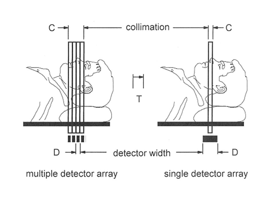
Multiple detector arrays

3. Xenon detectors
Use high-pressure (about 25 atm) nonradioactive xenon gas, in long thin cells between two metal plates
Very thick (e.g., 6 cm) to compensate in part for relatively low density
Thin metal septa separating individual detectors improves geometric efficiency by reducing dead space between detectors

5. Xenon detectors (cont.)
Long, thin plates are highly directional
Must be positioned in a fixed orientation with respect to the x-ray source
Cannot be used for 4th generation scanners because those detectors must record x-rays as the source moves over a wide angle

6. Solid-state detectors
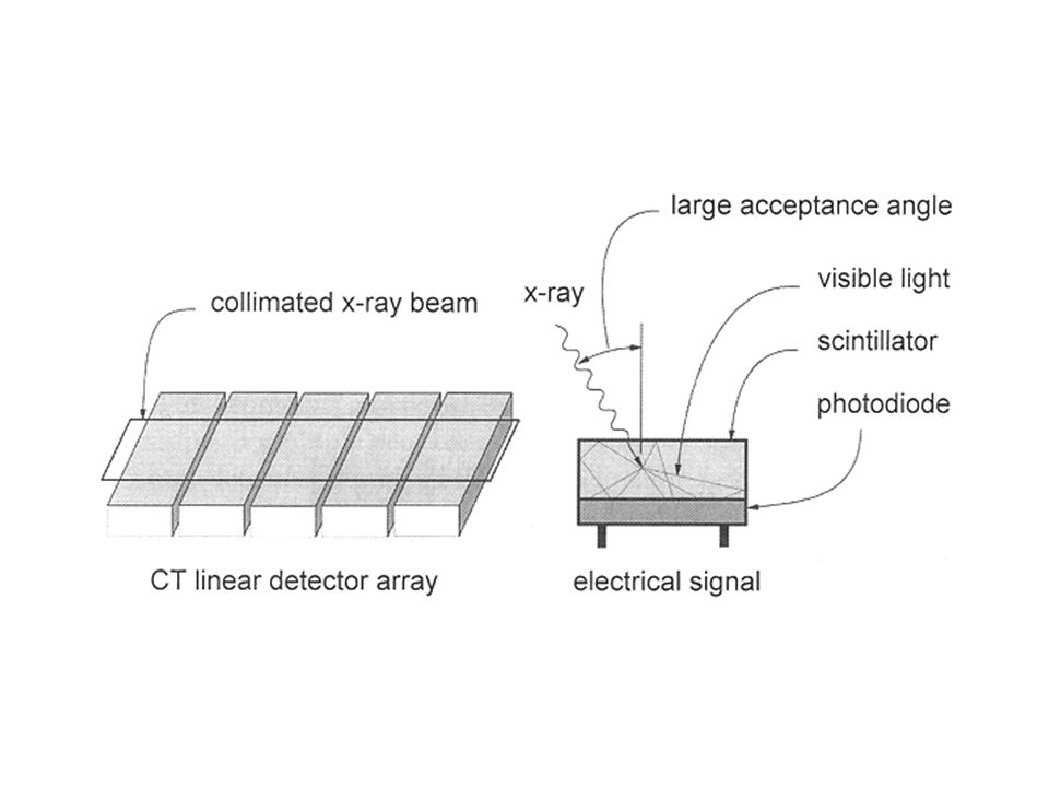
Composed of a scintillator coupled tightly to a photodetector (typically a photodiode)
Scintillator emits visible light when an x-ray is absorbed, similar to an x-ray intensifying screen
Photodetector converts light intensity into an electrical signal proportional to the light intensity

8. Solid-state detectors (cont.)
Detector size typically 1.0 x 15 mm (or 1.0 x 1.5 mm for multiple detector arrays)
Scintillators used include CdWO4 and yttrium and gadolinium ceramics
Better absorption efficiency than gas detectors because of higher density and higher effective atomic number

9. Solid-state detectors (cont.)
To reduce crosstalk between adjacent detector elements, a small gap between detector elements is necessary, reducing geometric efficiency somewhat
Top surface of detector is essentially flat and therefore capable of x-ray detection over a wide range of angles
Required for 4th generation scanners and used in most high-tier 3rd generation scanners as well

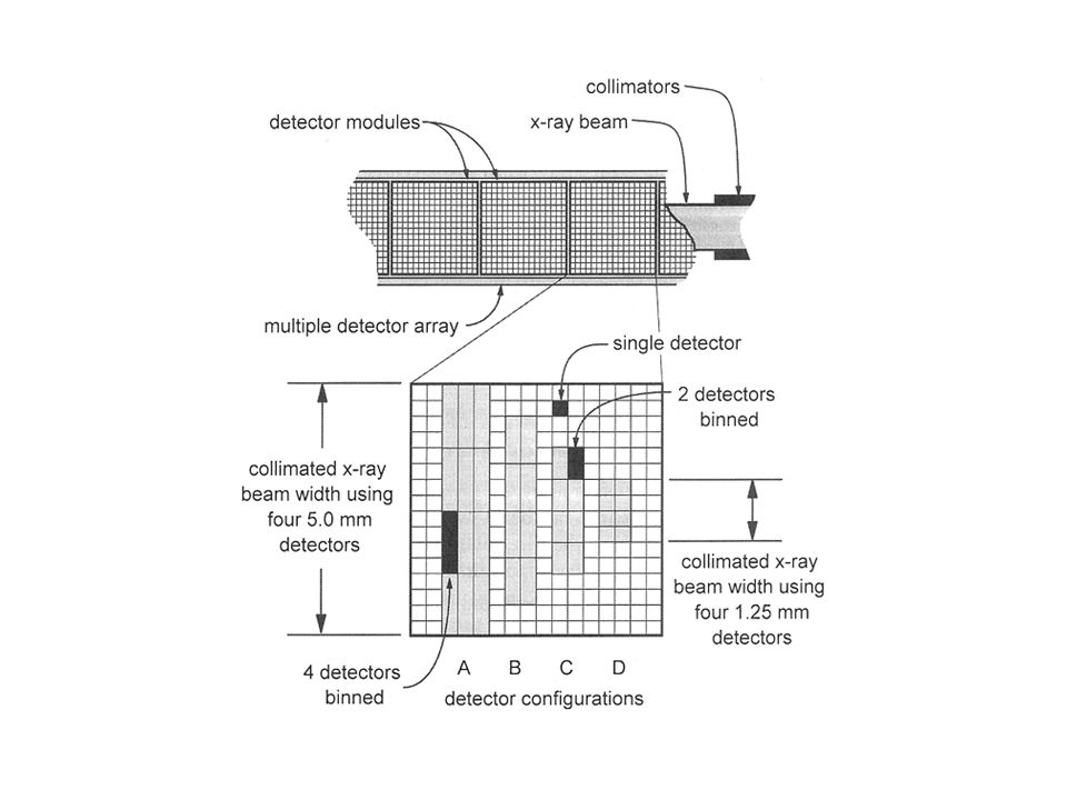
10. Multiple detector arrays
Set of several linear detector arrays, tightly abutted
Use solid-state detector arrays
Slice width is determined by the detectors, not by the collimator (although collimator does limit the beam to the total slice thickness)

12. Multiple detector arrays (cont.)
3rd generation multiple detector array with 16 detectors in the slice thickness dimension and 750 detectors along each array uses 12,000 individual detector elements
4th generation scanner would require roughly 6 times as many detector elements; consequently currently planned systems use 3rd generation geometry

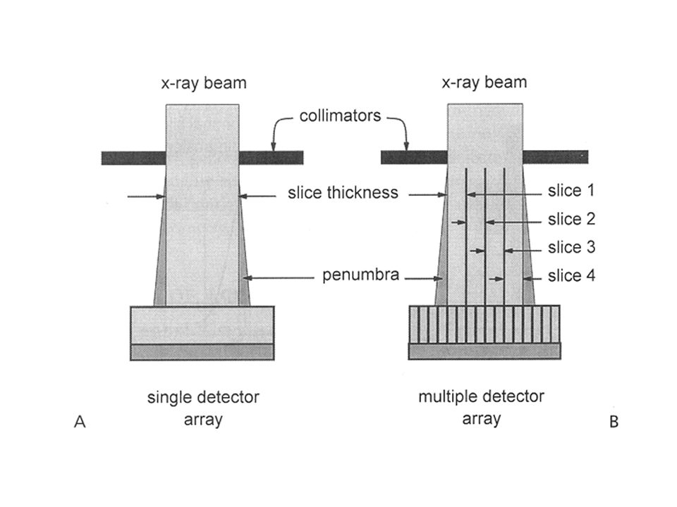
13. Slice thickness: single detector array scanners
Determined by the physical collimation of the incident x-ray beam with two lead jaws
Width of the detectors places an upper limit on slice thickness
For scans performed at the same kV and mAs, the number of detected x-ray photons increases linearly with slice thickness
Larger slice thicknesses yield better contrast resolution (higher SNR), but the spatial resolution in the slice thickness dimension is reduced

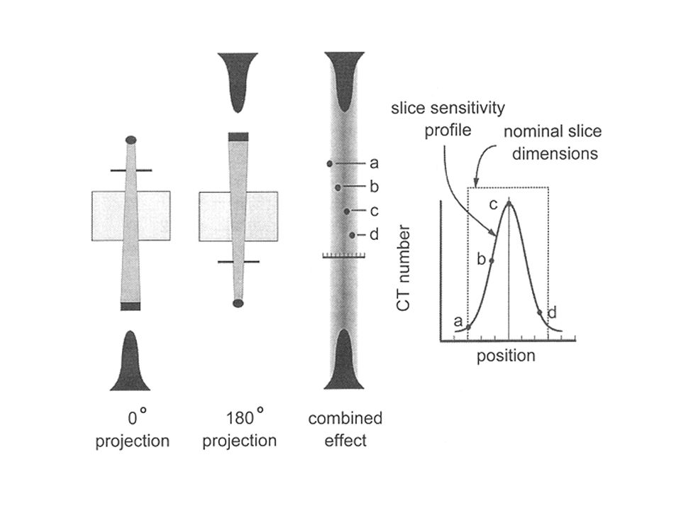
14. Slice sensitivity profile
For single detector array scanners, the shape of the slice sensitivity profile is a consequence of:
Finite width of the x-ray focal spot
Penumbra of the collimator
The fact that the image is computed from a number of projection angles encircling the patient
Other minor factors
Helical scans have a slightly broader slice sensitivity profile due to translation of the patient during the scan

16. Slice thickness: multiple detector array scanners
In axial scanning (i.e., with no table movement) where, for example, four detector arrays are used, the width of the two center detector arrays almost completely dictates the thickness of the slices
For the two slices at the edges of the scan, the inner side of the slice is determined by the edge of the detector, but the outer edge is determined either by the outer edge of the detector or by the collimator penumbra, depending on collimator adjustment

18. Slice thickness: MDA (cont.)
In helical mode, each detector array contributes to every reconstructed image
Slice sensitivity profile for each detector array needs to be similar to reduce artifacts
Typical to adjust the collimation so that the focal spot – collimator blade penumbra falls outside the edge detectors
Causes radiation dose to be a bit higher (especially for small slice widths)
Reduces artifacts by equalizing the slice sensitivity profiles between the detector arrays

19. Detector pitch/collimator pitch
Pitch is a parameter that comes into play when helical scan protocols are used
In a helical scanner with one detector array, the pitch is determined by the collimator
Collimator pitch = table movement (mm) per 360-degree rotation of gantry / collimator width (mm) at isocenter
Pitch may range from 0.75 (overscanning) to 1.5 (faster scan time, possibly smaller volume of contrast agent)

21. Pitch (cont.)
For scanners with multiple detector arrays, collimator pitch is still valid
Detector pitch = table movement (mm) per 360-degree rotation of gantry / detector width (mm)
For a multiple detector array scanner with N detector arrays, collimator pitch = detector pitch / N
For scanners with four detector arrays, detector pitches running from 3 to 6 are used

22. Tomographic reconstruction
Rays and views: the sinogram
Preprocessing the data
Interpolation (helical)

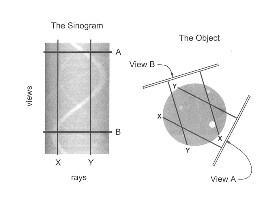
23. Sinogram
Display of raw data acquired for one CT slice before reconstruction
Rays are plotted horizontally and views are shown on the vertical axis
Objects close to the edge of the FOV produce a sinusoid of high amplitude
Bad detector in a 3rd generation scanner would show up as a vertical line on the sinogram

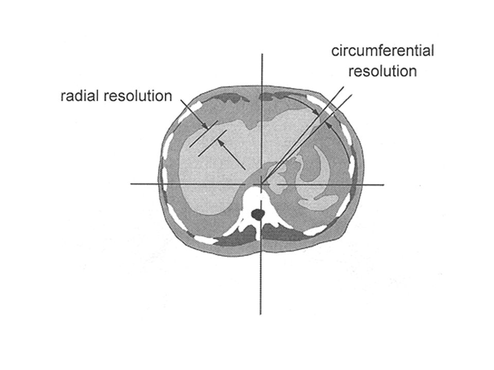
25. Rays and views
1st and 2nd generation scanners used 28,800 and 324,000 data points, respectively
State-of-the-art scanner may aquire about 800,000 data points
Modern 512 x 512 circular CT image contains about 205,000 image pixels
Number of rays affects the radial component of spatial resolution; number of views affects the circumferential component of the resolution

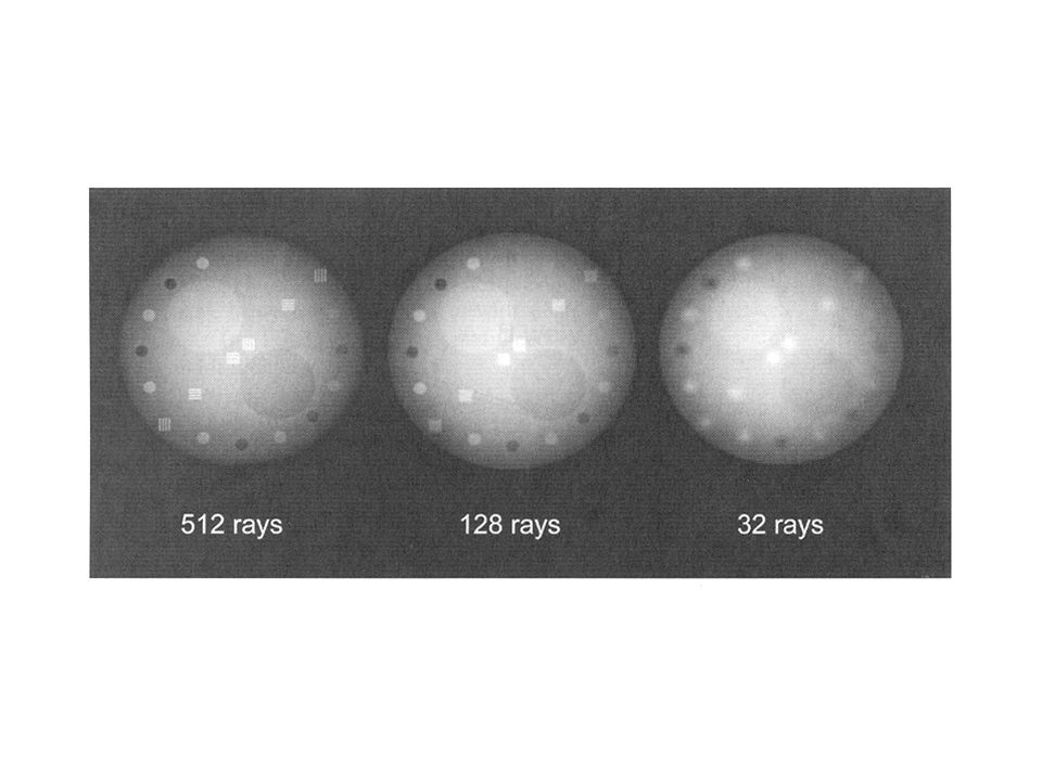
27. Number of rays
CT images of a simulated object reconstructed with differing numbers of rays show that reducing the ray sampling results in low-resolution, blurred images

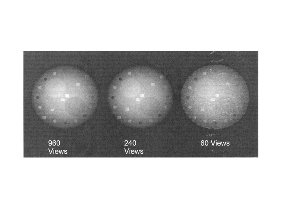
29. Number of views
CT images of the simulated object reconstructed with differing numbers of views show the effect of using too few angular views (view aliasing)
Sharp edges (high spatial frequencies) produce radiating artifacts that become more apparent near the periphery of the image

31. Preprocessing
Calibration data determined from air scans (performed by the technologist or service engineer periodically) provide correction data that are used to adjust the electronic gain of each detector
Variation in geometric efficiencies caused by imperfect detector alignments is also corrected

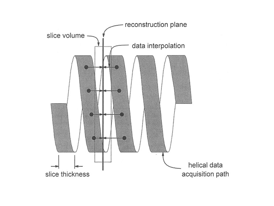
33. Interpolation
CT reconstruction algorithms assume that the x-ray source has negotiated a circular, not helical, path around the patient
Before the actual CT reconstruction, the helical data set is interpolated into a series of planar image sets
With helical scanning, CT images can be reconstructed at any position along the length of the scan

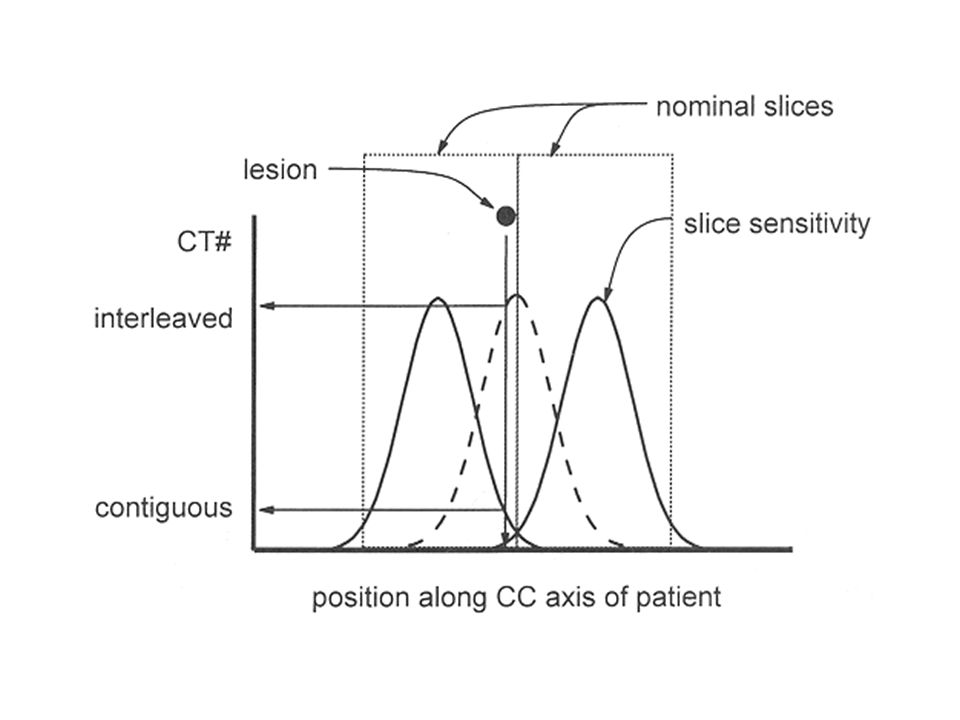
35. Interpolation (cont.)
Interleaved reconstruction allows the placement of additional images along the patient, so that the clinical examination is almost uniformly sensitive to subtle abnormalities
Adds no additional dose to the patient, but additional time is required to reconstruct the images
Actual spatial resolution along the long axis of the patient still dictated by slice thickness