1. Magnetic Resonance Imaging
Dr Sarah Wayte
University Hospital of Coventry & Warwickshire

3. Receiver Coils

4. ‘Typical’ MR Examination
Surface coil selected and positioned
Inside scanner for 20-30min
Series of images in different orientations & with different contrast obtained
It is very noisy

5. MRI in Cov & Warwickshire
Year
No of scanners
Field Strength
1987 1
0.5/1.0T
1997
1.0T
2001 2
1.0T, 1.5T
2002 3
2x1.5T, 1.0T
2006 6
5x1.5T, 1.0T

6. Coventry ‘Super’ Hospital
Opened July 2006
1.5T scanner (installed 2004 moved)
3.0T scanner (scanning June 07?)
0.35T open magnet (permanent magnet weighing 17.5tonnes, scanning Sept 07?)
(1.5T scanner in private hospital & 3 others in surrounding area)

7. Open 0.35T Ovation

8. What is so great about MRI
By changing imaging parameters (TR and TE times) can alter the contrast of the images
Can image easily in ANY plane (axial/sag/coronal) or anywhere in between

10. Resolution In slice resolution = Field of view / Matrix
Field of view typically 250mm head
Typical matrix 256
In slice resolution ~ 0.98mm
Slice thickness typically 3 to 5 mm
High resolution image
FOV=250mm, 512 matrix, in slice res~0.5mm
Slice thickness 0.5 to 1mm

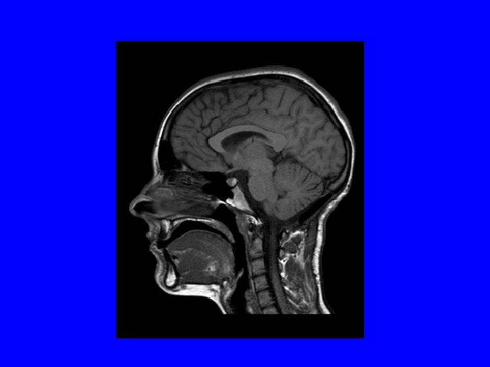
11. Any Plane
TR=2743ms TE=96ms
TR=498ms TE=12ms

12. Axial Slices Slice selection gradient applied from head to toe
Spins at various frequency from head to toe (fo=γBo)
RF pulse at fo gives slice through nose (resonance)
RF pulse at fo + f gives slice through eye
RF wave
fo+f fo fo - f
Slice selection gradient

13. Sagittal/Coronal Slices
Sagittal slice apply slice selection gradient left to right
Coronal slice apply slice selection gradient anterior to posterior
Combination of sag & coronal can give any angle between etc

14. Image Contrast
TR=525ms TE=15ms
TR=2500ms TE=85ms

15. Image Contrast Depends on the pulse sequence timings used
3 main types of contrast
T1 weighted
T2 weighted
Proton density weighted
Explain for 90 degree RF pulses

16. TR and TE
To form an image have to apply a series of 90o pulses (eg 256) and detect 256 signals
TR = Repetition Time = time between 90o RF pulses
TE = Echo Time = time between 90o pulse and signal detection TR TR
Signal Signal Signal TE TE TE

17. Bloch Equation Bloch Equations BETWEEN 90o RF pulses
Signal=Mo[1-exp(-TR/T1)] exp(-TE/T2)
TR<T1, TE<<T2, T1 weighted
TR~3T1, TE<T2, T2 weighted
TR~3T1, TE<<T2, Mo or proton density weighted TR TR
Signal Signal Signal TE TE TE

18. PD/T1/T2 Weighted Image T1 weighted Water dark Short TR=500ms
Short TE<30ms
T2 weighted
Water bright
Long TR=1500ms (3xT1max)
Long TE>80ms
PD weighted
Long TR=1500ms (3xT1max)
Short TE<30ms

19. T1/T2 Weighted Image
TR = 562ms
TE = 20ms
TR = 4000ms
TE = 132ms

20. T1/T2 Weighted
TR=525ms TE=15ms
TR=2500ms TE=85ms

21. Proton Density/T2
TR = 3070ms
TE = 15ms
TR = 3070ms
TE = 92ms

22. Proton Density/T2
TR = 3070ms
TE = 15ms
TR = 3070ms
TE = 92ms

23. Imaging Sequence: (Spin Warp)RF
time
Slice Selection Gradient
time
Phase Encoding Gradient
time
time
Frequency Encoding Gradient
Signal
time

24. K-Space ky
Phase Encoding kx

25. K-Space to Real Space ky 2D kx FT

26. K-Space to Real Space

27. Imaging Time (Spin Warp)
Imaging time = TR x matrix x Repetitions
Reps typically 2 or 4 (improves SNR)
E.g. TR=0.5s, Matrix=256, Reps=2
Image time = 256s = 4min 16s
During TR image other slices
Max no slices = TR/TE
e.g. 500/20=25 or 2500/120=21

28. Speeding Things Up 1
Spin warp T2 weighted image, 256 matrix, 3.5s TR, 2reps
Imaging time = 3.5 x 256 x 2 ~ 30min!!!
Solution, use 90_signal_signal_signal…. sequence of long TE time. Typical 21 signals per 90o pulse
Acquire 21 lines k-space per 90o pulse

29. Speeding Things Up 2
With 21 signals per 90o pulse for 256 matrix, 3.5s TR, 2reps
Imaging time = 3.5 x 256 x 2/21 ~ 1min 25s
All images I’ve shown so far use this technique
(Fast spin echo or turbo spin echo)

30. Echo Planar Imaging
Takes TSE/FSE to the extreme by acquiring 64 or 128 signals following a single 90 degree RF pulse
Image matrix size (64)2 or (128)2 (poor resolution)

31. Echo Planar Imaging ky
Phase Encoding kx
Frequency encoding

32. EPI Imaging Each slice acquired in 10s of mili-seconds
Lower resolution
More artefacts

33. EPI Imaging Each slice acquired in 10s of ms
Used as basis for functional MRI (fMRI)
Images acquired during ‘activation’ (e.g. finger tapping) and rest. Sum active and rest and subtract

34. EPI Imaging
Concentration of de-oxyhaemoglobin (longer T2* than oxyhaemoglobin) brighter
Subtracted image of bright ‘dots’ of activated brain
Super-impose dot image over ‘anatomical’ MR image
fMRI of candidate for epilepsy surgery.
Active area in verb generation task
Shows left-hemisphere localisation of language tasks

35. Diffusion Imaging
Uses EPI imaging technique with additional bi-polar gradients in x, y & z directions
Bi-polar gradients also varied in amplitude
No diffusion – high signal
More diffusion- lower signal

36. T2 & EPI Images: Stroke?

37. Different Amp Diffusion Gradient: Stroke?

38. Diffusion Direction
Diffusion gradient
Diffusion gradient

39. Diffusion Co-efficient Map : T2
Diffusion weighted image
T2 weighted image
Intensity α Diffusion
Intensity α T2

40. Propeller: Another method of sampling K-spaceky
Sampled k-space in rows so far
Propeller samples k-space in a ‘propeller’ pattern
Over-sampling centre k-space means in-sensitive to motion kx

41. Propeller Imaging
Propeller
Spin warp FSE

42. Propeller Gradients? ky kx

43. Inversion Recovery Sequence
This sequence has a 180o RF pulse which inverts all the magnetization before the standard 90o pulse and signal detection
TI = Inversion time = Time between 180o and 90o pulses TI TI
Signal Signal TR TE

44. Inversion Recovery Mz t
Fat
Brain
CSF t
Due to inverting 180o pulse, magnetization is recovering from a negative value Mz(t)=Mo[1-2exp(-TI/T1)]
With correct TI (1=2exp(-TI/T1) or TI=ln2T1) can eliminate signal from a tissue type completely

45. Inversion Recovery B0
Brain
CSF
Fat y y y x x x
180o inversion pulse

46. STIR = Short TI Inversion RecoveryMz
Fat
Brain
CSF t TI
TI= 130ms at 1.0T, so Mz of fat=O at this point> NO SIGNAL

47. STIR Flip 90 degrees Image with short TE Invert MagnetisationB0
Brain
CSF
Fat y y y x x x
Flip 90 degrees
Image with short TE
Invert Magnetisation
At Time TI
Fat at zero

48. STIR Image
TI=130ms
TR=4 450ms
TE=29ms

49. FLAIR Mz t FLAIR=Fluid Attenuated Inversion Recovery
Fat
Brain
CSF t TI
FLAIR=Fluid Attenuated Inversion Recovery
TI= 2500ms at 1.0T, so Mz of water=O at this point NO SIGNAL

50. FLAIR Flip 90 degrees Image with long TE Invert MagnetisationB0
Brain
CSF
Fat y y y x x x
Flip 90 degrees
Image with long TE
Invert Magnetisation
At Time TI
No Water Signal

51. FLAIR
TI=2500ms TR=9000ms TE=105ms
TR=2743ms TE=96ms

52. Even Faster Imaging How fast? 14-19images in a breath-hold
Use < 90 degree flip (α)
Some Mz magnetisation remains to form the next image, so TR<20ms
Drawback- less magnetisation/signal in transverse plane Mz
Signal = MoCosα

53. T1 Breath-hold Images 14 slices in 23s breath-hold (t1_fl2d_tra_bh)
TR=16.6ms, TE=6ms α=70o

54. T2 breath-hold images 19 slice in 25s breath-hold (t2-trufi_tra_bh)
TR=4.3ms TE=2.1ms α=80o

55. Dynamic Breast Tumour Imaging
Another fast imaging technique using <90 degree pulses
Acquire anatomical images to locate tumour
Acquire at 1min or 30s intervals, ( mm) images through the breast whilst injecting contrast agent
Draw region of interest over the tumour & look at how the contrast arrives and leaves the tumour

56. Breast Tumour Imaging

57. Imaging Blood Flow
Apply series of high flip angle pulses very quickly (short TR)
Stationary tissue does NOT have time to recover, becomes saturated
Flowing blood, seen no previous RF pulses, high signal from spins each time
Flip
Flip TR

58. MRA Base Images 72 slices through head
Brain tissue ‘saturated’ high signal from moving blood
Processed by computer to produce Maximum Intensity Projections (MIPs)
Maximum signal along line of site displayed

59. MIPs of Base Image

60. Abnormal MIP with AVM