1. Weak Lensing Tomography Sarah Bridle University College London

2. 3d vs 2d (tomography) Non-Gaussian -> higher order statistics Low redshift -> dark energy versus

3. Weak Lensing Tomography 1.In principle (perfect zs) Hu 1999 astro-ph/9904153 2.Photometric redshifts Csabai et al. astro-ph/0211080 3.Effect of photometric redshift uncertainties Ma, Hu & Huterer astro-ph/0506614 4.Intrinsic alignments 5.Shear calibration

4. 1. In principle (perfect zs) Qualitative overview Lensing efficiency and power spectrum –Dependence on cosmology Power spectrum uncertainties Cosmological parameter constraints

5. 1. In principle (perfect zs) Core reference Hu 1999 astro-ph/9904153 See also Refregier et al astro-ph/0304419 Takada & Jain astro-ph/0310125

6. Cosmic shear two point tomography  

7.  

8.   

9. 

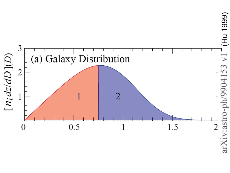
10. (Hu 1999)

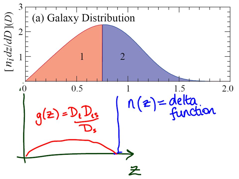
12. Lensing efficiency (Hu 1999) Equivalently: g i (z l ) = ∫ z l n i (z s ) D l D ls / D s dz s i.e. g is just the weighted D l D ls / D s

13. Can you sketch g 1 (z) and g 2 (z)? (Hu 1999) g i (z) = ∫ z s n i (z s ) D l D ls / D s dz s

14. Lensing efficiency for source plane?

16. (Hu 1999)

17. Sensitivity in each z bin

18. NOT

19. (Hu 1999) Why is g for bin 2 higher? A. More structure along line of sight B. Distances are larger g i (z d ) = ∫ z s 1 n i (z s ) D d D ds / D s dz s

21. * *

22. Lensing power spectrum (Hu 1999)

23. Lensing power spectrum Equivalently: P  ii (l) = ∫ g i (z l ) 2 P(l/D l,z) dD l /D l 2 i.e. matter power spectrum at each z, weighted by square of lensing efficiency (Hu 1999)

25. Measurement uncertainties 1/2 = rms shear (intrinsic + photon noise) n i = number of galaxies per steradian in bin i (Hu 1999) Cosmic Variance Observational noise

26. (Hu 1999)

27. Sensitivity in each z bin

28. NOT

29. (Hu 1999)

30. Dependence on cosmology Refregier et al SNAP3 ?? A.  m = 0.35 w=-1 B.  m = 0.30 w=-0.7

31. Approximate dependence Increase  8 → A. P  ↓ B. P  ↑ Increase z s → A. P  ↓ B. P  ↑ Increase  m → A. P  ↓ B. P  ↑ Increase  DE (  K =0) → A. P  ↓ B. P  ↑ Increase w → A. P  ↓ B. P  ↑ Huterer et al

32. Effect of increasing w on P  Distance to z –A. Decreases B. Increases

33. Perlmutter et al.1998 Fainter Further away Decelerating Accelerating  m =1, no DE  m =1,  DE =0) == (  m = 0.3,  DE = 0.7, w DE =0)

34. Perlmutter et al.1998 EdS OR w=0 w=-1 Fainter, further Brighter, closer

35. Effect of increasing w on P  Distance to z –A. Decreases B. Increases –When decrease distance, lensing effect decreases Dark energy dominates –A. Earlier B. Later

38. Effect of increasing w on P  Distance to z –A. Decreases B. Increases –When decrease distance, lensing decreases Dark energy dominates –A. Earlier B. Later Growth of structure –A. Suppressed B. Increased –Lensing A. Increases B. Decreases Net effects: –Partial cancellation decreased sensitivity –Distance wins

39. Approximate dependence Increase  8 → A. P  ↓ B. P  ↑ Increase z s → A. P  ↓ B. P  ↑ Increase  m → A. P  ↓ B. P  ↑ Increase  DE (  K =0) → A. P  ↓ B. P  ↑ Increase w → A. P  ↓ B. P  ↑ Huterer et al

40. Approximate dependence Increase  8 → A. P  ↓ B. P  ↑ Increase z s → A. P  ↓ B. P  ↑ Increase  m → A. P  ↓ B. P  ↑ Increase  DE (  K =0) → A. P  ↓ B. P  ↑ Increase w → A. P  ↓ B. P  ↑ Huterer et al Note modulus

41. Which is more important? Distance or growth? Simpson & Bridle

42. Dependence on cosmology Refregier et al SNAP3 ?? A.  m = 0.35 w=-1 B.  m = 0.30 w=-0.7

43. (Hu 1999)

44. See Heavens astro-ph/0304151 for full 3D treatment (~infinite # bins)

45. (Hu 1999)

46. Parameter estimation for z~2 (Hu 1999)

47. Predict the direction of degeneracy in w versus  m plane

48. Refregier et al SNAP3

49. (Hu 1999)

50. Takada & Jain

51. (Hu 1999)

52. Covariance matrix P 12 is correlated with P 11 and P 22 (ignoring trispectrum contributions) Takada & Jain

54. How many redshift bins to use? Ma, Hu & Huterer 5 is enough Modified from

55. Higher order statistics

56. Takada & Jain

58. Geometric information Jain & Taylor; Kitching et al. Slide stolen from Tom Kitching www.astro.dur.ac.uk/Cosmology/SISCO/edin_talks/Kitching.PPT

59. Slide stolen from presentation by Andy Taylor www.shef.ac.uk/physics/idm2004/talks/monday/originals/taylor_andy.ppt

60. Slide stolen from presentation by Andy Taylor www.shef.ac.uk/physics/idm2004/talks/monday/originals/taylor_andy.ppt

61. Slide stolen from presentation by Andy Taylor www.shef.ac.uk/physics/idm2004/talks/monday/originals/taylor_andy.ppt

62. Slide stolen from presentation by Andy Taylor www.shef.ac.uk/physics/idm2004/talks/monday/originals/taylor_andy.ppt

63. Some additional tomographic methods Cross-correlation cosmography –Bernstein & Jain astro-ph/0309332 Galaxy-lensing cross correlation –Hu & Jain astro-ph/0312395 Reconstruction of distance and growth –Song; Knox & Song