Download presentation
Presentation is loading. Please wait.

1
卜磊 bulei@nju.edu.cn Transition System

2
Part I: Introduction Chapter 0: Preliminaries Chapter 1: Language and Computation Part II: Models Chapter 2: Finite Automata Chapter 3: Regular Expressions Chapter 4: Context-Free Grammars Chapter 5: Pushdown Automata Chapter 6: Turing Machines

3
Part III: Modeling Chapter 7: Transition Systems Chapter 8: Petri Nets, Time Petri Nets Chapter 9: Timed Automata, Hybrid Automata Chapter 10: Message Sequence Charts Part IV: Model Checking and Tools Chapter 11: Introduction of Model Checking Chapter 12: SPIN Model Checker Chapter 13: UPPAAL: a model-checker for real-time systems Chapter 14:…

4
7.1 Definitions and notations Reactive System The intuition is that a transition system consists of a set of possible states for the system and a set of transitions - or state changes - which the system can effect. When a state change is the result of an external event or of an action made by the system, then that transition is labeled with that event or action. Particular states or transitions in a transition system can be distinguished.

5
model to describe the behavior of systems digraphs where nodes represent states, and edges model transitions state: the current color of a traffic light the current values of all program variables + the program counter the value of register and output transition: (“state change”) a switch from one color to another the execution of a program statement the change of the registers and output bits for a new input
 a switch from one color to another the execution of a program statement the change of the registers and output bits for a new input")
7
Transition systems

8
Paths

13
Labeled transition systems

16
Traces

17
Relation

18
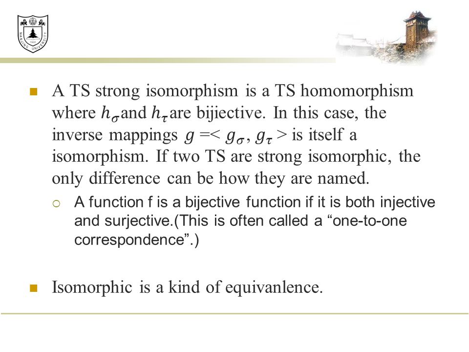
There are numerous notions of equivalency for transition systems We consider the following: Strong isomorphism Weak isomorphism Bisimulation equivalence

19
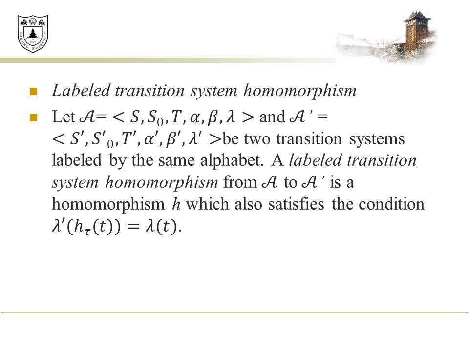
Transition system homomorphism

23
Are these two systems isomorphic?

24
Weak Isomorphism

25
These two systems are weak isomorphic Theorem: If two transition systems are isomorphic, then they are weakly isomorphic. Weak isomorphism is an equivalence relation

27
Example two isomorphic TS are bisimilar, but bisimilar TS are not necessarily isomorphic

28
The lady or the tiger

29
Strong Isomorphism: the transition systems are identical except for the names of the states. Weak Isomorphism: the transition systems are strongly isomorphic provided that the transition systems are restricted to the reachable states. Bisimulation Equivalence: the transition systems have the same behavior, and make choice at same time.

30
Use TS to present the behavior of all the modeling language Then Use TS to prove the equivalence respectively

31
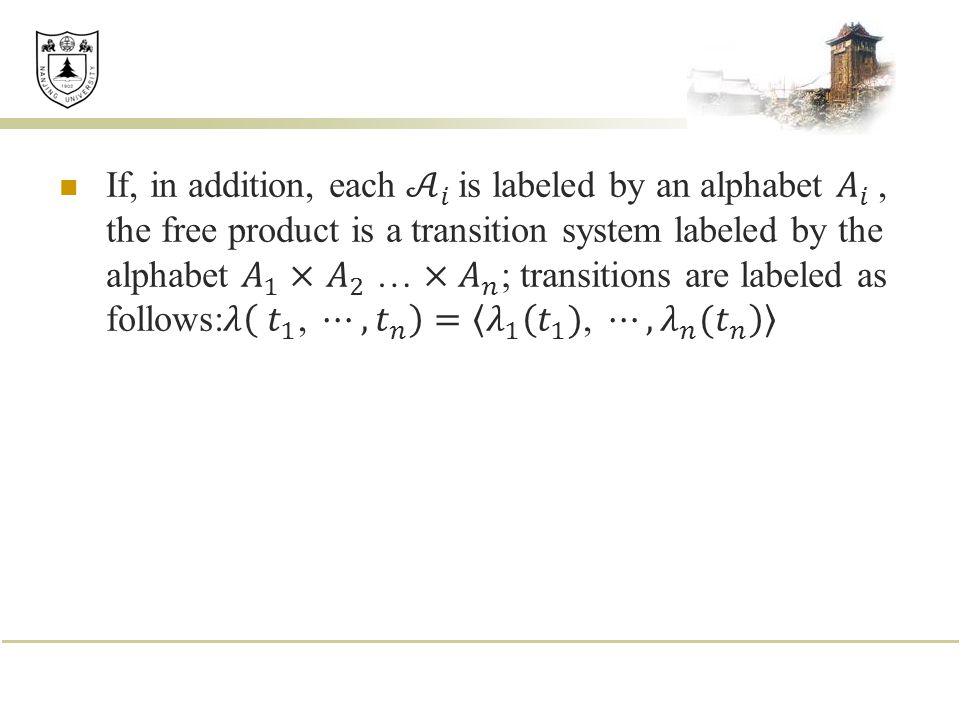
The free product of transition systems

32
p q s t p,s p,t q,s q,t

35
The free product assumes that in a global system, all component systems execute their transitions simultaneously, it is possible to divide time into intervals in such a way that during each of those intervals each component executes exactly one transition. In other words, the same ‘clock’ drives the different transition systems forming the product.

36
The synchronous product of transition systems When processes interact, not all possible global actions are useful, since the interaction is subject to communication and synchronization constraints. The transition system associated with the system of processes must therefore be a subsystem of the free product of the component transition systems. The communication and synchronization constraints that define the subsystem can always be simply expressed by the synchronous product, formally defined below.

38
p q s t p,s p,t q,k q,t k p,k q,s

39
a b c p q s t p,s p,t q,k q,t k p,k q,s

40
a b c p q s t p,s p,t q,k q,t k p,k q,s

41
p q s t p,s p,t q,s q,t

42
Shared label

43
Modeling sequential circuits

45
A Mutual Exclusion Protocol Two concurrently executing processes are trying to enter a critical section without violating mutual exclusion

46
State Space The state space of a program can be captured by the valuations of the variables and the program counters For our example, we have two program counters: pc1, pc2, domains of the program counters: {out, wait, cs} three boolean variables: turn, a, b, boolean domain: {True, False} Each state of the program is a valuation of all the variables

47
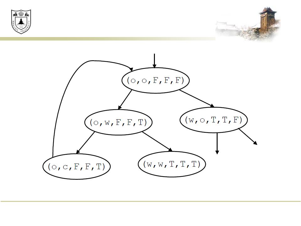
Each state can be written as a tuple (pc1,pc2,turn,a,b) Initial states: {(o,o,F,F,F), (o,o,F,F,T), (o,o,F,T,F), (o,o,F,T,T), (o,o,T,F,F), (o,o,T,F,T), (o,o,T,T,F), (o,o,T,T,T)} – initially: pc1=o and pc2=o How many states total? 3 * 3 * 2 * 2 * 2 = 72 exponential in the number of variables and the number of concurrent components

48
Transition Relation specifies the next-state relation, i.e., given a state what are the states that can come immediately after that state For example, given the initial state (o,o,F,F,F) Process 1 can execute: out: a := true; turn := true; or Process 2 can execute: out: b := true; turn := false; If process 1 executes, the next state is (w,o,T,T,F) If process 2 executes, the next state is (o,w,F,F,T) So the state pairs ((o,o,F,F,F),(w,o,T,T,F)) and ((o,o,F,F,F),(o,w,F,F,T)) are included in the transition relation
 Process 1 can execute: out: a := true; turn := true; or Process 2 can execute: out: b := true; turn := false; If process 1 executes, the next state is (w,o,T,T,F) If process 2 executes, the next state is (o,w,F,F,T) So the state pairs ((o,o,F,F,F),(w,o,T,T,F)) and ((o,o,F,F,F),(o,w,F,F,T)) are included in the transition relation")
50
P =m: cobegin P 0 || P 1 coend m’ P 0 :: l 0 : while True do NC 0 : wait (turn =0); CR 0 : turn :=1; end while l 0 ’ P 1 : l 1 : while True do NC 1 : wait (turn =1); CR 1 : turn :=0; end while l 1 ’
; CR 0 : turn :=1; end while l 0 ’ P 1 : l 1 : while True do NC 1 : wait (turn =1); CR 1 : turn :=0; end while l 1 ’")
52
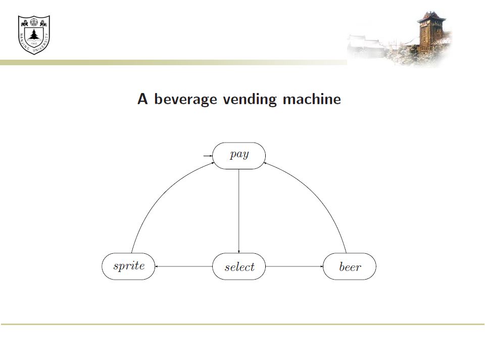
Temporal Properties once r is 1, it will be 1 forever Two program cannot in the critical section together If you choose sprite, you cannot get beer unless you pay again No deadlock

53
Introduction Temporal logic is a formalism for describing sequences of transitions between states in a reactive system. Properties like eventually or never are specified using special temporal operators. CTL* Software Engineering Group 53

55
CTL* CTL* formulas describe properties of computation trees. The computation tree shows all of the possible executions starting from the initial state. Software Engineering Group 55

56
Path quantifiers and Temporal operators Path quantifiers: A ( for all computation path ) E ( for some computation path ) Temporal operators: X, F, G, U, R Software Engineering Group 56
 E ( for some computation path ) Temporal operators: X, F, G, U, R Software Engineering Group 56")
57
X (next time) requires the property holds in the second state of the path F (eventually) the property will hold at some state on the path G (always) the property holds at every state on the path U (until) if there is a state on the path where the second property holds, at every preceding state, the first one holds R (release) the second property holds along the path up to and including the first state where the first property holds. However, the first property is not required to hold eventually

58
two types of formulas in CTL* state formulas ( which are true in a special state ) path formulas ( which are true along a special path ) syntax of state formulas rules: if then p is sf if f and g are sf, are sf if f is a pf, then E f and A f are sf Software Engineering Group 58
 path formulas ( which are true along a special path ) syntax of state formulas rules: if then p is sf if f and g are sf, are sf if f is a pf, then E f and A f are sf Software Engineering Group 58")
59
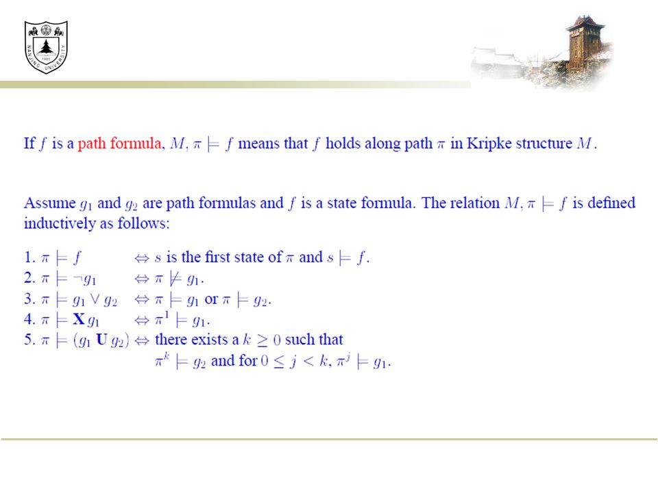
syntax of path formulas: if f is a sf, then f is also a pf if f and g are pf,, X f, F f, G f, f U g and f R g are pf CTL* is the set of state formulas generated by the above rules semantics of CTL* if f is a sf, M, s ->f means that f holds at state s in the M if g is a pf, M, π-> g means that g holds along path π in the M Software Engineering Group 59

62
CTL and LTL two sublogics of CTL* branching-time logic the temporal operators quantify over the paths that are possible from a given state. Temporal operators must be immediately preceded by a path quantifier. if f and g are sf, X f, F f, G f, f U g and f R g are pf A(FG p) Linear temporal logic operators are provided for describing events along a single computation path. LTL implicitly quantifies universally over paths. If, then p is pf, Af where f is a pf AG(EF p) Software Engineering Group 62
 Linear temporal logic operators are provided for describing events along a single computation path. LTL implicitly quantifies universally over paths. If, then p is pf, Af where f is a pf AG(EF p) Software Engineering Group 62.")
63
CTL ten basic CTL operators: AX and EX AF and EF AG and EG AU and EU AR and ER Software Engineering Group 63

64
Each of the ten operators can be expressed in terms of EX, EG and EU AX f= ! EX(!f) EF f= E[True U f] AG f =!EF(!f) AF f= !EG(!f) A[f U g]= !E[!gU(!f ^ !g)] ^ !EG !g A[f R g] = !E[!f U !g] E[f R g] = !A[!f U !g]
 EF f= E[True U f] AG f =!EF(!f) AF f= !EG(!f) A[f U g]= !E[!gU(!f ^ !g)] ^ !EG !g A[f R g] = !E[!f U !g] E[f R g] = !A[!f U !g].")
65
CTL Software Engineering Group 65

66
Examples Let "P" mean "I like chocolate" and Q mean "It's warm outside." AG.P "I will like chocolate from now on, no matter what happens.“ EF.P "It's possible I may like chocolate some day, at least for one day." AF.EG.P "It's always possible (AF) that I will suddenly start liking chocolate for the rest of time." (Note: not just the rest of my life, since my life is finite, while G is infinite). EG.AF.P "This is a critical time in my life. Depending on what happens next (E), it's possible that for the rest of time (G), there will always be some time in the future (AF) when I will like chocolate. However, if the wrong thing happens next, then all bets are off and there's no guarantee about whether I'll ever like chocolate." Software Engineering Group 66
, it s possible that for the rest of time (G), there will always be some time in the future (AF) when I will like chocolate. However, if the wrong thing happens next, then all bets are off and there s no guarantee about whether I ll ever like chocolate. Software Engineering Group 66.")
67
A(PUQ) "From now until it's warm outside, I will like chocolate every single day. Once it's warm outside, all bets are off as to whether I'll like chocolate anymore. Oh, and it's guaranteed to be warm outside eventually, even if only for a single day." E((EX.P)U(AG.Q)) "It's possible that: there will eventually come a time when it will be warm forever (AG.Q) and that before that time there will always be some way to get me to like chocolate the next day (EX.P)." Software Engineering Group 67
U(AG.Q)) It s possible that: there will eventually come a time when it will be warm forever (AG.Q) and that before that time there will always be some way to get me to like chocolate the next day (EX.P). Software Engineering Group 67.")
68
Express Properties Safety: something bad will not happen Typical examples: AG ( reactor_temp > 1000 ) Usually: AG Software Engineering Group 68
 Usually: AG Software Engineering Group 68")
69
Express Properties Liveness: something good will happen Typical examples: AF( rich ) AF( x > 5 ) AG( start -> AF terminate ) Usually: AF Software Engineering Group 69
 AF( x > 5 ) AG( start -> AF terminate ) Usually: AF Software Engineering Group 69")
70
Express Properties Fairness: something is successful/allocated infinitely often. Typical examples: AGAF ( enabled ) Usually: AGAF Software Engineering Group 70
 Usually: AGAF Software Engineering Group 70.")
71
Software Engineering Group 71

Similar presentations

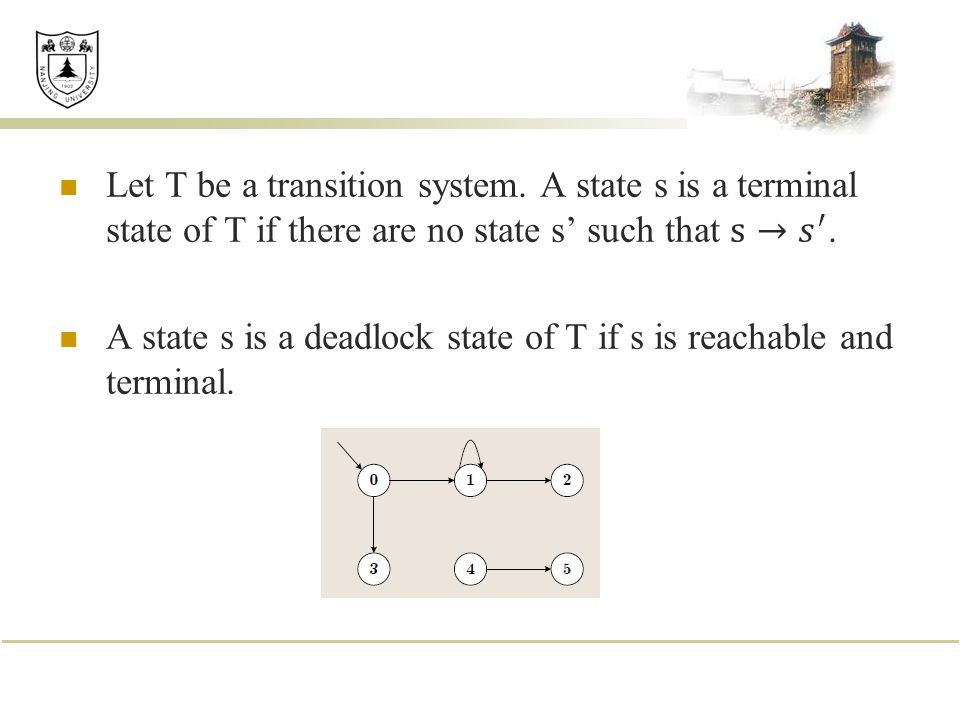


 and a property (in some temporal logic) Outputs: Decision about whether or not the property always holds.>")

