1. BASIS OF M/EEG SIGNAL Maciej Cosilo Panagiotis Papagiannopoulos

2. Electroencephalography (EEG)

3. History Richard Caton (1842-1926) from Liverpool, in the British Medical Journal in 1875 reported: „ Feeble currents of varying direction pass through the multiplier when electrodes are placed on two points of the external surface [of the brain], or one electrode on the grey matter and one on the surface of the skul...” In 1890 Adolf Beck: spontaneous electrical activity in response to light in rabbits and dogs- not really knowing about Caton’s findings. In 1912 Vladimir Vladimirovich Pravdich-Neminsky published the first animal EEG study on evoked potential in the mammalian brain. In 1914 polish physiologist Napoleon Cybulski (Beck’s collaborator) and Jelenska-Macieszyna photographed EEG recordings of experimentally induced seizures.

4. History

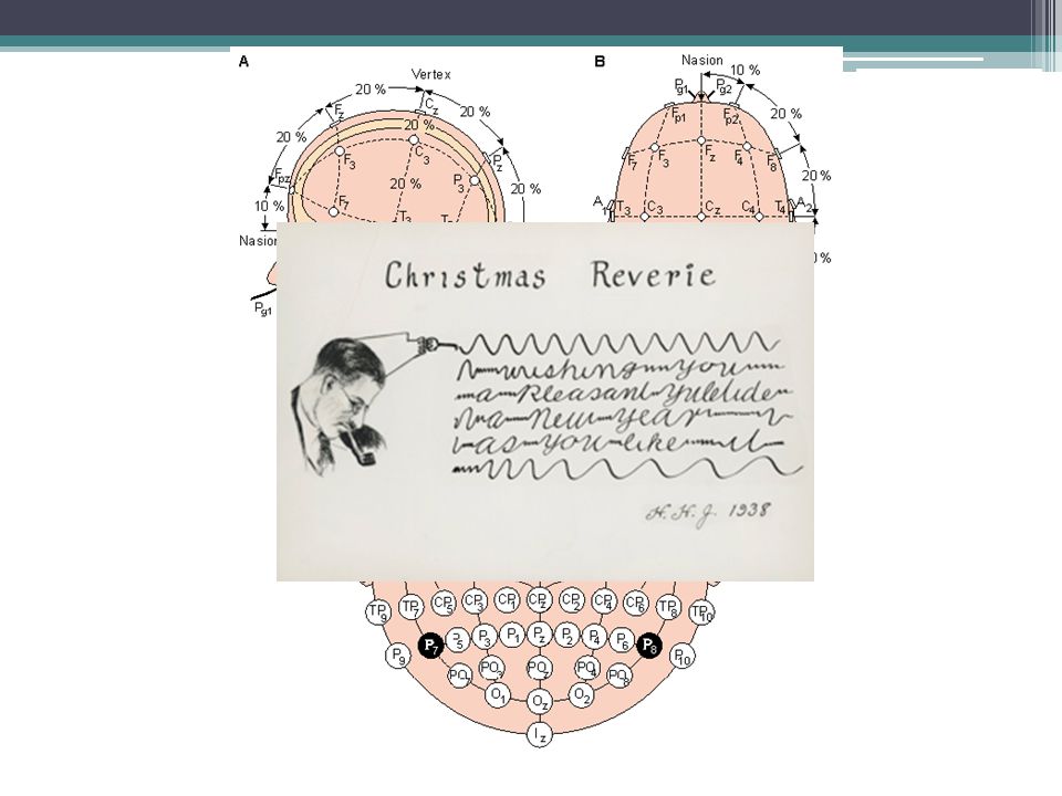
5. Instrumentation Active electrodes placed on scalp. Arrangement: 10-20 system (by Herbert Jasper)

7. Instrumentation Active electrodes placed on scalp. Arrangement: 10-20 system (by Herbert Jasper) Number of electrodes can vary: 32, 64,128 or 256 electrodes (richer data, but not necessarily better?) Signal is amplified and converted to digital form. Voltage is a potential for current to move from one point to another.

8. You can’t really say you’re measuring voltage at a single site. EEG reflects a potential for current to pass between two electrodes. Reference montage: EEG represents a difference in voltage between an active electrode and a reference electrode. Cz, ear lobes, mastoids, tip of the nose, toe (!). Average Reference montage: Averaged voltage of all the electrodes used as a reference. Need a high density of electrodes for this. Electrode Input 1 Electrode Input 2 EEG waveform= Input1 – Input 2 Amplifier Instrumentation

9. Graphic representation of voltage difference between two cortical areas, plotted against time. Continuous, spontaneous EEG

11. Electrical activity in the brain Two main sources of electrical activity: ▫ Action potentials ▫ Post-synaptic potentials

12. Action Potentials Action potentials Action potentials ▫ Discrete, rapid voltage spikes. If two neurons fire at the same time, the voltages will summate and the voltage recorded at electrodes will be twice as large. Timing issue:Timing issue: If a neuron 1 fires after neuron 2, the current at a given location will be flowing into one axon at the same time that it is flowing out of the other axon. In effect, they “cancel” each other, and the recorded voltage is much smaller. Neurons rarely fire at the same time.

13. Membrane equilibrium (resting) potential of about -70mV Ion channels on the post- synaptic membrane open or close in response to neurotransmitters binding to the receptors. Flow of Na+ inward the cell depolarizes postsynaptic neuron. Flow of Cl- inward hyperpolarizes postsynaptic neuron. Post- synaptic potentials

14. Excitatory Post- Synaptic Potential: Due to the flow of ions, extracellular electrode detects negative voltage difference (current sink is generated) The current flows further down the cell, completing a loop, where Na+ flow outside the cell. Extracellular electrode detects positive voltage difference A dipole is generated Post- synaptic potentials

15. Pyramidal neurons are spatially aligned and perpendicular to the cortical surface. Similar orientation, receiving similar input. Ideal candidate for a current generator

16. Artifacts Environmental artifacts Changes in electrode impedance External electrical noise Physiological artifacts Blinks Eye movements Muscle artifacts

17. Averaging EEG analysis: Event- related potentials

18. Time- Frequency Analysis Neurons oscillate at different frequencies Time- frequency analysis allows to tell which frequencies contribute to the recorded activity, and how they change over time Example: induced gamma-band frequency related to perceptual binding C. Tallon- Baundry & O. Bertrand, Trends Cogn. Sci, 1999

19. Volume conduction: transmission of electrical current from its source, through the conductors (brain tissue) towards measurement device (EEG electrodes) Measured voltage will depend on the orientation of the dipole and resistance of brain, skull, scalp, eye holes. Volume conduction & The inverse problem

21. Volume conduction: transmission of electrical current from its source, through the conductors (brain tissue) towards measurement device (EEG electrodes) Measured voltage will depend on the orientation of the dipole and resistance of brain, skull, scalp, eye holes. Current does not simply flow between two poles of the dipole Rather, it spreads throughout the conductor Thus, activity is “blurred”- potentials generated in one part of the brain are recordable at distant parts of the scalp as well. Volume conduction & The inverse problem

22. This creates a problem- if you give me a voltage distribution, I will not be able to tell the location of the dipoles, because there is an infinite number of dipoles that can produce any given voltage distribution (The “Inverse Problem”). We can try to solve the Inverse Problem by trying to go the other way around! We can place a source of activity in a specific place in a brain model, and calculate how the distribution would look like for that given dipole. Then, we can compare it with the actual activity to see if it matches our model. Thus, we can solve the inverse problem by applying a forward model. (Not as easy as it sounds, especially for the EEG!) Volume conduction & The inverse problem

23. BASIS OF MEG SIGNAL

24. A brief history 1968: David Cohen measures the first (noisy) magnetic brain signal 1970: James Zimmerman invents the ‘Superconducting Quantum Interference Device (SQUID) 1972:Cohen performs the first (1 sensor) MEG recording based on one SQUID detector 80s: Multiple sensors into arrays to cover a larger area Present–day: typically contain 300 sensors, covering most of the head 1968: David Cohen measures the first (noisy) magnetic brain signal 1970: James Zimmerman invents the ‘Superconducting Quantum Interference Device (SQUID) 1972:Cohen performs the first (1 sensor) MEG recording based on one SQUID detector 80s: Multiple sensors into arrays to cover a larger area Present–day: typically contain 300 sensors, covering most of the head

25. MEG Instrumentation ????????? Acts as refrigerant Insulating storage vessel Shielded room

26. What is this? A very sensitive magnetometer used to measure extremely subtle magnetic fields It is sensitive enough to measure fields as low as 5x10 -8 T A small ring (2-3mm) of superconducting material What does it look like…? A very sensitive magnetometer used to measure extremely subtle magnetic fields It is sensitive enough to measure fields as low as 5x10 -8 T A small ring (2-3mm) of superconducting material What does it look like…? S uperconducting Qu antum I nterference D evice

27. SQUID

28. How does it work? When the SQUID is immersed in liquid helium (4.2K), it becomes superconducting. As a consequence, current can flow across the junction via the process of conducting tunneling The current is modulated in a very sensitive fashion by the external magnetic field threading the loop. This makes the SQUID the most sensitive magnetic field detector known!!!!!!!! When the SQUID is immersed in liquid helium (4.2K), it becomes superconducting. As a consequence, current can flow across the junction via the process of conducting tunneling The current is modulated in a very sensitive fashion by the external magnetic field threading the loop. This makes the SQUID the most sensitive magnetic field detector known!!!!!!!!

29. The squid is very small to collect much of magnetic flux. Larger pick-up coils are used to collect the magnetic field over a relatively large area. By means of inductive coupling, the coils funnel the measured flux into the SQUID ring. The squid is very small to collect much of magnetic flux. Larger pick-up coils are used to collect the magnetic field over a relatively large area. By means of inductive coupling, the coils funnel the measured flux into the SQUID ring. …and what’s the role of pick-up coils?

30. What do we measure with MEG? Electromagnetic activity (magnetic component) 1. S ynchronous activation 2. S pecific geometry 3. S trength of the field (decreases with square distance) But… is it possible for the action potentials to fire in a synchronous fashion?

31. What do we measure with MEG?  primary currents/secondary currents  MEG is more sensitive to primary currents

32. Supp_Motor_Area Parietal_Sup Frontal_Inf_Oper Occipital_Mid Frontal_Med_Orb Calcarine Heschl Insula Cingulum_Ant ParaHippocampal Hippocampus Putamen Amygdala Caudate Cingulum_Post Brainstem Thalamus STN Cornwell et al. 2008; Riggs et al. 2009 Hung et al. 2010; Cornwell et al. 2007, 2008 Parkonen et al. 2009 Timmerman et al. 2003 RMS Lead field Over subjects and voxels MEG Sensitivity to depth

33. The forward Problem WHAT IS THE FORWARD PROBLEM FOR? The first step for the reconstruction of the spatial- temporal activity of the neural sources of the MEG (and EEG) data.

34. How do we solve the forward problem? 1.Computing the external magnetic fields at a finite set of sensor locations and orientations (channel configuration)… given a predefined set of source positions and orientations (source configuration). 2.Using simple conductivity models – “head” models (geometry)

35. 1. Computing the external magnetic field… n, orientation r, location Θ, orientation r q, location q, magnitude A convenient algebraic formulation of the MEG forward model (Mosher et al., 1999) SENSOR SOURCE B, data L, Lead field (matrix), the forward solution in each source, field distribution across all M channels S, source

36. 2.Using different “head” models (conductivity & geometry) Finite Element Method (FEM) Boundary Element Method (BEM) Multiple Spheres Single Sphere Simpler models

37. 2.Using different “head” models (conductivity & geometry) Single Sphere model Assumptions: 1. Head as a set of nested concentric spheres (brain, CSF, skull, scalp) 2. Each layer has uniform and constant conductivity * The analytic approach for the forward problem

38. 2.Using different “head” models (conductivity & geometry) Boundary Element Method Real geometry and conductivity Usage of MRI, X Ray give anatomical information Accurate conductivity parameters required Hundred megabytes A lot of time… and money! * The numerical approach for the forward problem

39. EEGMEG Electrical signal Deep & shallow: radial and tangential sources Tricky to localize A relatively cheap technique Electrical signal Deep & shallow: radial and tangential sources Tricky to localize A relatively cheap technique Magnetic signal Mostly shallow: tangential sources Easier to obtain and localize But expensive Magnetic signal Mostly shallow: tangential sources Easier to obtain and localize But expensive Both: excellent temporal resolution

40. Thank you!