1. Ludovico Biagi & Athanasios Dermanis Politecnico di Milano, DIIAR Aristotle University of Thessaloniki, Department of Geodesy and Surveying Crustal Deformation Analysis from Permanent GPS Networks European Geophysical Union General Assembly - EGU2009 19 -24 April 2009, Vienna, Austria

2. Our approach - Departure from classical horizontal deformation analysis:

3. - New rigorous equations for deformation invariant parameters: Principal (max-min) linear elongation factors & their directions Dilatation, (maximum) shear strain & its direction

4. Our approach - Departure from classical horizontal deformation analysis: - New rigorous equations for deformation invariant parameters: Principal (max-min) linear elongation factors & their directions Dilatation, (maximum) shear strain & its direction - New rigorous equations for “horizontal” deformation analysis on the reference ellipsoid Attention: NOT for the physical surface of the earth, NOT 3-dimentional !

5. Our approach - Departure from classical horizontal deformation analysis: - New rigorous equations for deformation invariant parameters: Principal (max-min) linear elongation factors & their directions Dilatation, (maximum) shear strain & its direction - Separation of relative rigid motion of (sub)regions from actual deformation: Identification of regions with different kinematic behavior (clustering) Use of best fitting reference system for each region (Concept of regional discrete Tisserant reference system) - New rigorous equations for “horizontal” deformation analysis on the reference ellipsoid Attention: NOT for the physical surface of the earth, NOT 3-dimentional !

6. Our approach - Departure from classical horizontal deformation analysis: - New rigorous equations for deformation invariant parameters: Principal (max-min) linear elongation factors & their directions Dilatation, (maximum) shear strain & its direction - Separation of relative rigid motion of (sub)regions from actual deformation: Identification of regions with different kinematic behavior (clustering) Use of best fitting reference system for each region (Concept of regional discrete Tisserant reference system) - New rigorous equations for “horizontal” deformation analysis on the reference ellipsoid Attention: NOT for the physical surface of the earth, NOT 3-dimentional ! PLUS Study of signal-to-noise ratio (significance) of deformation parameters from spatially interpolated GPS velocity estimates using: - Finite element method (triangular elements) - Minimum Mean Square Error Prediction (collocation) CASE STUDY: Central Japan

7. Deformation as comparison of tw o shapes (at two epochs) x = coordinates at epoch t Mathematical Elasticity: Deformation studied via the deformation gradient local linear approximation to the deformation function

8. Deformation as comparison of tw o shapes (at two epochs) x = coordinates at epoch t u = x - x = displacements Mathematical Elasticity: Deformation studied via the deformation gradient local linear approximation to the deformation function Geophysics-Geodesy: Deformation studied via the displacement gradient and approximation to strain tensor

9. Classical horizontal deformation analysis A short review

10. Classical horizontal deformation analysis Strain tensor E : description of (quadratic) variation of length element

11. Classical horizontal deformation analysis Strain tensor E : description of (quadratic) variation of length element Geodetic data: Discrete initial coordinates x 0i and velocities v i at GPS permanent stations P i Displacements: u i = (t – t 0 ) v i

12. SPATIAL INTERPOLATION for the determination of or Classical horizontal deformation analysis Strain tensor E : description of (quadratic) variation of length element Geodetic data: Discrete initial coordinates x 0i and velocities v i at GPS permanent stations P i Displacements: u i = (t – t 0 ) v i Require: DIFFERENTIATION for the determination of or

13. Discrete geodetic information at GPS permanent stations Classical horizontal deformation analysis

14. Discrete geodetic information at GPS permanent stations Interpolation to obtain continuous information, e.g. displacements at every point Classical horizontal deformation analysis SPATIAL INTERPOLATION

15. Discrete geodetic information at GPS permanent stations Interpolation to obtain continuous information, e.g. displacements at every point Differentiation to obtain the deformation gradient F or displacement gradient J = F - I Classical horizontal deformation analysis SPATIAL INTERPOLATION

16. Analysis of the displacement gradient J into symmetric and antisymmetric part: Classical horizontal deformation analysis

17. Analysis of the displacement gradient J into symmetric and antisymmetric part:  = small rotation angle Classical horizontal deformation analysis

18. Analysis of the displacement gradient J into symmetric and antisymmetric part: diagonalization e max, e min = principal strains  = direction of e max  = small rotation angle Classical horizontal deformation analysis

19. Analysis of the displacement gradient J into symmetric and antisymmetric part: diagonalization  = small rotation angle  = dilataton  = maximum shear strain  = direction of   Classical horizontal deformation analysis e max, e min = principal strains  = direction of e max

20. Analysis of the displacement gradient J into symmetric and antisymmetric part: diagonalization  = small rotation angle  = dilataton  = maximum shear strain  = direction of   Classical horizontal deformation analysis e max, e min = principal strains  = direction of e max

21. SVD Horizontal deformational analysis using the Singular Value Decomposition (SVD) A new approach

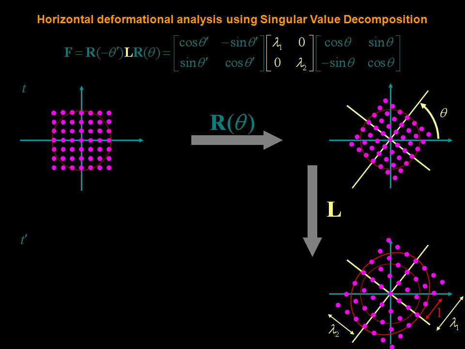
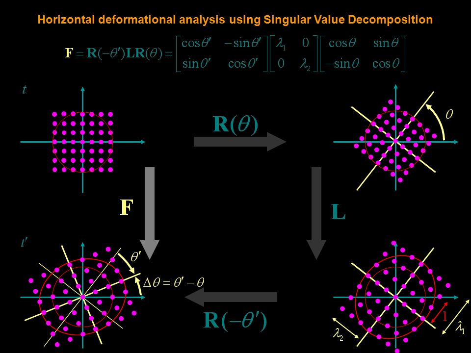
22. Horizontal deformational analysis using Singular Value Decomposition from diagonalizations: SVD

23. Horizontal deformational analysis using Singular Value Decomposition

28. Rigorous derivation of invariant deformation parameters without the approximations based on the infinitesimal strain tensor

29. Rigorous derivation of invariant deformation parameters shear along the 1st axis linear scale factordirection of shear additional rotation not contributing to deformation 2 alternative 4-parametric representations

30. Rigorous derivation of invariant deformation parameters shear along the 1st axis linear scale factordirection of shear additional rotation not contributing to deformation 2 alternative 4-parametric representations

31. Rigorous derivation of invariant deformation parameters shear along the 1st axis linear scale factordirection of shear additional rotation not contributing to deformation 2 alternative 4-parametric representations

32. Rigorous derivation of invariant deformation parameters shear along the 1st axis linear scale factordirection of shear additional rotation not contributing to deformation 2 alternative 4-parametric representations

33. Rigorous derivation of invariant deformation parameters shear along the 1st axis linear scale factordirection of shear additional rotation not contributing to deformation 2 alternative 4-parametric representations

34. Rigorous derivation of invariant deformation parameters shear along the 1st axis linear scale factordirection of shear additional rotation not contributing to deformation 2 alternative 4-parametric representations

35. shear along the 1st axis Rigorous derivation of invariant deformation parameters

36. shear along direction  Rigorous derivation of invariant deformation parameters

37. additional rotation  (no deformation) Rigorous derivation of invariant deformation parameters

38. additional scaling (scale factor s) Rigorous derivation of invariant deformation parameters

39. Compare the two representations and express s, , ,  as functions of 1, 2, ,  Rigorous derivation of invariant deformation parameters

40. Derivation of dilatation 

41. Use Singular Value Decomposition and replace Rigorous derivation of invariant deformation parameters Derivation of shear , and its direction 

42. Rigorous derivation of invariant deformation parameters Derivation of shear , and its direction  Compare

43. Rigorous derivation of invariant deformation parameters Derivation of shear , and its direction 

44. Rigorous derivation of invariant deformation parameters Derivation of shear , and its direction 

45. Horizontal deformation on the surface of the reference ellipsoid

46. Actual deformation is 3-dimensional Horizontal deformation on ellipsoidal surface

47. But we can observe only on 2-dimensional earth surface ! Horizontal deformation on ellipsoidal surface

48. Why not 3D deformation? 3D deformation requires not only interpolation but also an extrapolation outside the surface Extrapolation from surface geodetic data is not reliable – requires additional geophysical hypothesis INTERPOLATION EXTRAPOLATION Horizontal deformation on ellipsoidal surface

49. Standard horizontal deformation: Project surface points on horizontal plane, Study the deformation of the derived (abstract) planar surface Horizontal deformation on ellipsoidal surface

50. Why not study deformation of actual earth surface? Local surface deformation is a view of actual 3D deformation through a section along the tangent plane to the surface. For variable terrain: we look on 3D deformation from different directions ! Horizontal and vertical deformation caused by different geophysical processes (e.g. plate motion vs postglacial uplift) Horizontal deformation on ellipsoidal surface

51. Our approach to horizontal deformation: Project surface points on reference ellipsoid, Study the deformation of the derived (abstract) ellipsoidal surface Horizontal deformation on ellipsoidal surface

52. Use curvilinear coordinates on the surface (geodetic coordinates) Formulate coordinate gradient HOW IT IS DONE: Horizontal deformation on ellipsoidal surface

53. HOW IT IS DONE: F q refers to local (non orthonormal) coordinate bases: Horizontal deformation on ellipsoidal surface

54. HOW IT IS DONE: F q refers to local (non orthonormal) coordinate bases: Change to orthonormal bases: converting metric matrices to identity Horizontal deformation on ellipsoidal surface

55. HOW IT IS DONE: F q refers to local (non orthonormal) coordinate bases: Change to orthonormal bases: Transform F q to orthonormal bases: converting metric matrices to identity Horizontal deformation on ellipsoidal surface

56. HOW IT IS DONE: THEN PROCEED AS IN THE PLANAR CASE

57. Separation of rigid motion from deformation The concept of the discrete Tisserant reference system best adapted to a particular region

58. Separation of rigid motion from deformation SPATIAL INTERPOLATION

59. Separation of rigid motion from deformation

60. BAD SPATIAL INTERPOLATION Separation of rigid motion from deformation

61. GOOD SPATIAL INTERPOLATION PIECEWISE INTERPOLATION INVOLVES DISCONTINUITIES = FAULTS ! Separation of rigid motion from deformation

62. Horizontal Displacements Separation of rigid motion from deformation

63. Horizontal Displacements Separation of rigid motion from deformation

64. Different displacements behavior in 3 regions Apart from internal deformation regions are in relative motion Separation of rigid motion from deformation

65. HOW TO REPRESENT THE MOTION OF A DEFORMING REGION AS A WHOLE ? BY THE MOTION OF A REGIONAL OPTIMAL REFERENCE SYSTEM ! OPTIMAL = SUCH THAT THE CORRESPONDING DISPLACEMENTS (OR VELOVITIES) BECOME AS SMALL AS POSSIBLE Separation of rigid motion from deformation

66. ORIGINAL REFERENCE SYSTEM OPTIMAL REFERENCE SYSTEM Motion as whole ( = motion of reference system) + internal deformation ( = motion with respect to the reference system) Separation of rigid motion from deformation

67. Horizontal motion on earth ellipsoid (  sphere): Rotation around an axis with angular velocity  Separation of rigid motion from deformation

68. Horizontal motion on earth ellipsoid (  sphere): Rotation around an axis with angular velocity  DEFINITION OF OPTIMAL FRAME: Minimization of relative kinetic energy of regional network Discrete Tisserant reference system Separation of rigid motion from deformation

69. Horizontal motion on earth ellipsoid (  sphere): Rotation around an axis with angular velocity  DEFINITION OF OPTIMAL FRAME: Minimization of relative kinetic energy of regional network Discrete Tisserant reference system Separation of rigid motion from deformation SOLUTION: = inertia matrix = relative angular momentum Migrating pole, variable angular velocity versus usual constant rotation (Euler rotation)

70. Spatial interpolation or prediction

71. TRIANGULAR FINITE ELEMENTSMINIMUM MEAN SQUARE ERROR PREDICTION (COLLOCATION) Spatial interpolation or prediction true interpolated true interpolated

72. TRIANGULAR FINITE ELEMENTSMINIMUM MEAN SQUARE ERROR PREDICTION (COLLOCATION) Spatial interpolation or prediction Deterministic interpolationInterpolation by stochastic prediction true interpolated true interpolated

73. TRIANGULAR FINITE ELEMENTSMINIMUM MEAN SQUARE ERROR PREDICTION (COLLOCATION) Spatial interpolation or prediction Piecewise linear displacements Piecewise constant deformation parameters Continuous displacements Continuous deformation parameters Deterministic interpolationInterpolation by stochastic prediction true interpolated true interpolated

74. TRIANGULAR FINITE ELEMENTSMINIMUM MEAN SQUARE ERROR PREDICTION (COLLOCATION) Spatial interpolation or prediction Piecewise linear displacements Piecewise constant deformation parameters Continuous displacements Continuous deformation parameters Observation errors completely absorbed in deformation parameters estimates Observation errors partially removed by interpolation smoothing Deterministic interpolationInterpolation by stochastic prediction true interpolated true interpolated

75. TRIANGULAR FINITE ELEMENTSMINIMUM MEAN SQUARE ERROR PREDICTION (COLLOCATION) Spatial interpolation or prediction Piecewise linear displacements Piecewise constant deformation parameters Continuous displacements Continuous deformation parameters Observation errors completely absorbed in deformation parameters estimates Observation errors partially removed by interpolation smoothing Deterministic interpolationInterpolation by stochastic prediction Accuracy estimates of deformation parameters reflect only data uncertainty Accuracy estimates of deformation parameters reflect both data and interpolation uncertainty true interpolated true interpolated

76. Principal linear elongation factors vs principal strains A comparison

77. Linear elongations and strains StrainsLinear elongation factors Definitions

78. Linear elongations and strains StrainsLinear elongation factors Definitions Computation from diagonalizations

79. Linear elongations and strains StrainsLinear elongation factors Meaning ? clear meaning ! Definitions Computation from diagonalizations Interpretation

80. Linear elongations and strains StrainsLinear elongation factors Meaning ? clear meaning ! Definitions Computation from diagonalizations Interpretation Relation

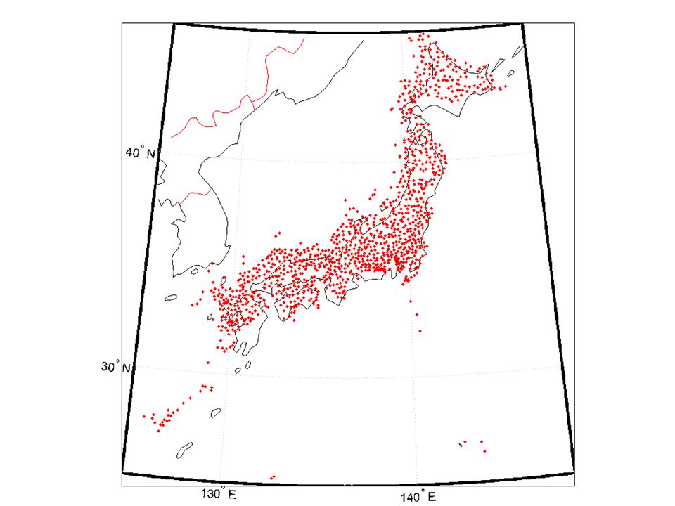
81. Case study: National permanent GPS network in Central Japan

83. Case study: Central Japan Original velocities

84. Reduced velocities (removal of rotation) Case study: Central Japan

85. Reduced velocities

86. Case study: Central Japan Division in 3 regions. Relative velocities w.r. region R2 after removal of rigid rotations

87. Linear elongation factors max = 1, min = 2 FINITE ELEMENTS SEPARATE COLLOCATIONS IN EACH REGION

88. Dilatation  and shear  FINITE ELEMENTSCOLLOCATION

89. SNR = Signal to Noise Ration FINITE ELEMENTS COLLOCATION

90. FINITE ELEMENTS COLLOCATION SNR = Signal to Noise Ration

91. Linear trends in each sub-region ( max -1)  10 6 0.002  0.006 ( min -1)  10 6  0.044  0.008  57.1  6.0   10 6  0.043  0.010   10 6 0.046  0.010  12.1  6.0 ( max -1)  10 6 0.004  0.007 ( min -1)  10 6  0.072  0.008  89.6  3.9   10 6  0.068  0.011   10 6 0.076  0.011  134.6  3.9 ( max -1)  10 6  0.001  0.013 ( min -1)  10 6  0.116  0.021  69.5  5.8   10 6  0.117  0.024   10 6 0.116  0.026  24.5  5.8 R1 R2 R3 R1 R2 R3

92. Conclusions Minimum Mean Square Error Prediction (collocation) has the following advantages: - Produces continuous results for any desired point in the region of application -Provides smooth results where the effect of the data errors is partially removed - Provides more realistic variances-covariances which in addition to the data uncertainty reflect also the interpolation uncertainty

93. THANKS FOR YOUR ATTENTION A copy of this presentation can be downloaded from http://der.topo.auth.gr/