1. Geometry Compression Michael Deering, Sun Microsystems SIGGRAPH (1995) Presented by: Michael Chung

2. Geometry Compression What is it? Lossy technique for reducing the size of geometry representation.

3. Motivation Save bandwidth and transmission time in graphics accelerators and networks. Save storage space in main memory and on disk.

4. Proposed Contributions Technique for lossy compression ratios of between 6 and 10 to 1 –Claims only slight losses in object quality –Depends on original representation format and final quality level desired

5. Geometry Compression What is it? Trade-off between quality (subjective) and amount of compression. Compression steps can be reversed for decompression

6. Geometry Compression What is it? Goal: represent geometry with geometry compression instructions

7. Insights Reduce size of geometry representation in several ways. –Reuse vertices in triangle strip via reference –Bit shaving –Geometry is local, encode deltas –Normals as indices

8. Compression Steps 1.Convert triangle data to generalized triangle mesh 2.Quantization of positions, colors, normals 3.Delta encoding of quantized values 4.Huffman tag-based variable-length encoding of deltas 5.Output binary output stream with Huffman table initializations and geometry compression instructions

9. Compression Steps 1.Convert triangle data to generalized triangle mesh 2.Quantization of positions, colors, normals 3.Delta encoding of quantized values 4.Huffman tag-based variable-length encoding of deltas 5.Output binary output stream with Huffman table initializations and geometry compression instructions

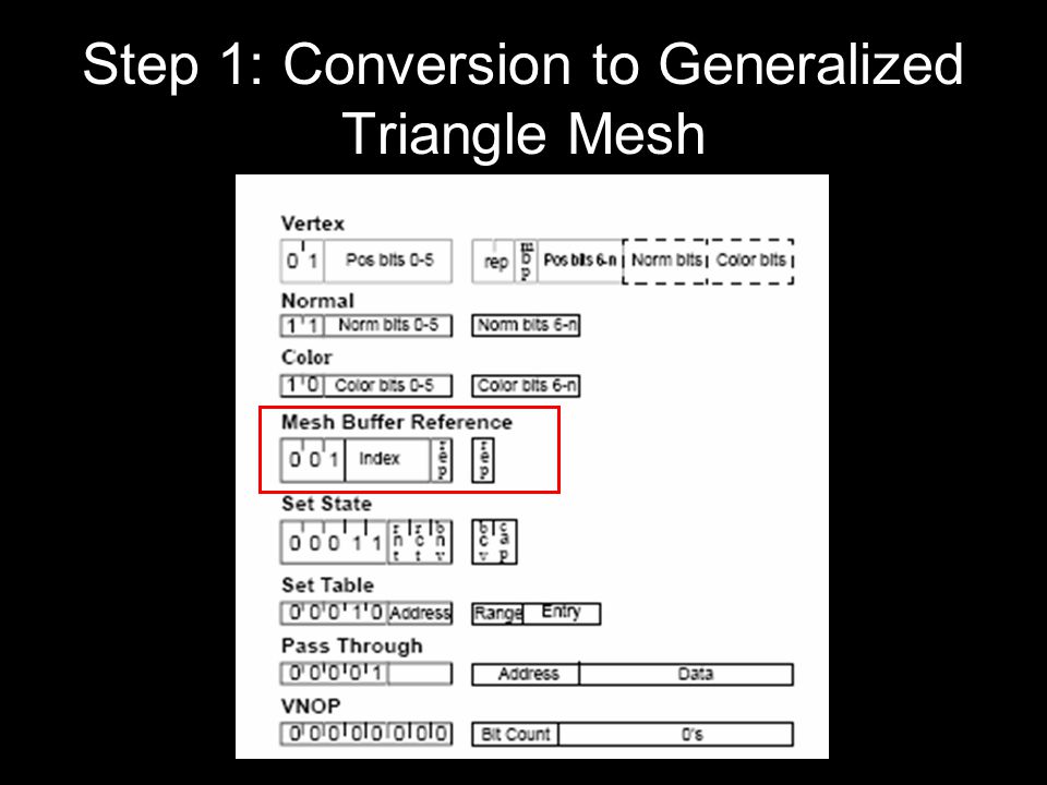
10. Step 1: Conversion to Generalized Triangle Mesh generalized triangle strip  generalized triangle mesh Generalized triangle strip –Specifies vertices with four vertex replacement codes (2 bits): Replace oldest Replace middle Restart clockwise Restart counterclockwise

11. Step 1: Conversion to Generalized Triangle Mesh Generalized triangle strip (example)

12. Step 1: Conversion to Generalized Triangle Mesh Generalized triangle strip (example)

13. Step 1: Conversion to Generalized Triangle Mesh Generalized triangle strip (example)

14. Step 1: Conversion to Generalized Triangle Mesh Generalized triangle strip (example)

15. Step 1: Conversion to Generalized Triangle Mesh Generalized triangle strip (example)

16. Step 1: Conversion to Generalized Triangle Mesh Generalized triangle strip (example)

17. Step 1: Conversion to Generalized Triangle Mesh Generalized triangle strip (example)

18. Step 1: Conversion to Generalized Triangle Mesh Generalized triangle strip (example)

19. Step 1: Conversion to Generalized Triangle Mesh Generalized triangle strip (example)

20. Geometry Compression Instruction Set

23. Step 1: Conversion to Generalized Triangle Mesh generalized triangle strip  generalized triangle mesh Generalized triangle mesh –Generalized triangle strip –Mesh buffer 16 slot queue 4 bit index Explicitly push vertices onto mesh buffer for reuse. –We save because only 4 bits are required to reference old vertex.

24. Step 1: Conversion to Generalized Triangle Mesh Generalized triangle mesh (example)

25. Step 1: Conversion to Generalized Triangle Mesh Generalized triangle mesh (example)

26. Step 1: Conversion to Generalized Triangle Mesh Generalized triangle mesh (example)

27. Step 1: Conversion to Generalized Triangle Mesh Generalized triangle mesh (example)

28. Step 1: Conversion to Generalized Triangle Mesh Generalized triangle mesh (example)

29. Step 1: Conversion to Generalized Triangle Mesh Generalized triangle mesh (example)

30. Step 1: Conversion to Generalized Triangle Mesh Generalized triangle mesh (example)

31. Step 1: Conversion to Generalized Triangle Mesh Generalized triangle mesh (example)

32. Step 1: Conversion to Generalized Triangle Mesh Generalized triangle mesh (example)

33. Step 1: Conversion to Generalized Triangle Mesh Generalized triangle mesh (example)

34. Step 1: Conversion to Generalized Triangle Mesh Generalized triangle mesh (example)

35. Step 1: Conversion to Generalized Triangle Mesh Generalized triangle mesh (example)

36. Step 1: Conversion to Generalized Triangle Mesh

38. Geometry Compression Instruction Set

39. Compression Steps 1.Convert triangle data to generalized triangle mesh 2.Quantization of positions, colors, normals 3.Delta encoding of quantized values 4.Huffman tag-based variable-length encoding of deltas 5.Output binary output stream with Huffman table initializations and geometry compression instructions

40. Step 2: Quantization

42. Some parts of the geometry may require more or less precision than others.

43. Step 2: Quantization Some parts of the geometry may require more or less precision than others. So, the amount of quantization we perform per position, normal, and color is variable.

44. Step 2: Quantization Position –32-bit floating-point coordinates are wasteful. 8-bit exponent allows an unnecessary range of values. 24-bit fixed-point mantissa offers unnecessary precision.

45. Step 2: Quantization Position –Based on empirical visual tests, allow at most 16 bits per component (X, Y, Z)

46. Step 2: Quantization Color –Linear reflectivity values R, G, B, (optional) A Range from 0.0 to 1.0 per component cap state bit sets alpha ON and OFF –At most 12 unsigned fraction bits per component

47. Geometry Compression Instruction Set

48. Step 2: Quantization Normal –96 bits can represent up to 2 96 different normals We don’t need so many –Angular density of 0.01 radians between normals visually indistinguishable This is about 100,000 normals distributed over a unit sphere 48 bits to represent a normal (16 bits per X, Y, Z) –We can do better than 48 bits per normal Use clever indexing to represent ~100,000 normals with 18 bits…

49. Step 2: Quantization Normal –96 bits can represent up to 2 96 different normals We don’t need so many –Angular density of 0.01 radians between normals visually indistinguishable This is about 100,000 normals distributed over a unit sphere 48 bits to represent a normal (16 bits per X, Y, Z) –We can do better than 48 bits per normal Use clever indexing to represent ~100,000 normals with 18 bits…

50. Step 2: Quantization Normal –96 bits can represent up to 2 96 different normals We don’t need so many –Angular density of 0.01 radians between normals visually indistinguishable This is about 100,000 normals distributed over a unit sphere 48 bits to represent a normal (16 bits per X, Y, Z) –We can do better than 48 bits per normal Use clever indexing to represent ~100,000 normals with 18 bits…

51. Step 2: Quantization Normal –Take advantage of symmetry About 100,000 unit normals distributed across unit sphere Split unit sphere into 48 symmetrical parts

52. Step 2: Quantization –3 bits to specify octant –3 bits to specify sextant within octant –All normals in sextant (~2000) stored in a table Two orthogonal angular addresses index into table At most 6 bits per angular index –Grand total: 6 – 18 bit index per normal

53. Step 2: Quantization –3 bits to specify octant –3 bits to specify sextant within octant –All normals in sextant (~2000) stored in a table Two orthogonal angular addresses index into table At most 6 bits per angular index –Grand total: 6 – 18 bit index per normal

54. Step 2: Quantization –3 bits to specify octant –3 bits to specify sextant within octant –All normals in sextant (~2000) stored in a table Two orthogonal angular addresses index into table At most 6 bits per angular index –Grand total: 6 – 18 bit index per normal

55. Step 2: Quantization –What about the 26 normals at the shared corners of each sextant? These normals belong to more than one sextant, but should be represented only once –3-bit indices 110 and 111 have not been assigned to a sextant Use one of these indices to represent the unique collection of these 26 normals

56. Step 2: Quantization –What about the 26 normals at the shared corners of each sextant? These normals belong to more than one sextant, but should be represented only once –3-bit indices 110 and 111 have not been assigned to a sextant Use one of these indices to represent the unique collection of these 26 normals

57. Step 2: Quantization –Angular indices represent a regular grid of coordinates in angular space

58. Step 2: Quantization –Angular indices represent a regular grid of coordinates in angular space

59. Step 2: Quantization –Angular indices represent a regular grid of coordinates in angular space

60. Step 2: Quantization Summary –Position: 16 bits or less per component –Color: 12 bits or less per component –Normal: 6 – 18 bits total 6 bits to take advantage of symmetry 0 – 12 bits to index table of normals per sextant

61. Compression Steps 1.Convert triangle data to generalized triangle mesh 2.Quantization of positions, colors, normals 3.Delta encoding of quantized values 4.Huffman tag-based variable-length encoding of deltas 5.Output binary output stream with Huffman table initializations and geometry compression instructions

62. Step 3: Delta Encoding Represent components with deltas between neighbors

63. Step 3: Delta Encoding

64. Represent components with deltas between neighbors

65. Step 3: Delta Encoding Represent components with deltas between neighbors Store histogram of delta group bit lengths –One histogram per group type (position, normal, color)

66. Compression Steps 1.Convert triangle data to generalized triangle mesh 2.Quantization of positions, colors, normals 3.Delta encoding of quantized values 4.Huffman tag-based variable-length encoding of deltas 5.Output binary output stream with Huffman table initializations and geometry compression instructions

67. Huffman Encoding Huffman encoding assigns shorter tags to more frequently encountered data.

68. Huffman Encoding Huffman encoding assigns shorter tags to more frequently encountered data.

69. Huffman Encoding Huffman encoding assigns shorter tags to more frequently encountered data.

70. Huffman Encoding Huffman encoding assigns shorter tags to more frequently encountered data.

71. Huffman Encoding Huffman encoding assigns shorter tags to more frequently encountered data.

72. Huffman Encoding Huffman encoding assigns shorter tags to more frequently encountered data.

73. Step 4: Huffman Tag-Based Variable-Length Encoding Assign a Huffman tag to each delta encoded position, normal, or color. The tag encodes the bit length of the associated delta data.

74. Compression Steps 1.Convert triangle data to generalized triangle mesh 2.Quantization of positions, colors, normals 3.Delta encoding of quantized values 4.Huffman tag-based variable-length encoding of deltas 5.Output binary output stream with Huffman table initializations and geometry compression instructions

75. Geometry Compression Instruction Set

76. Binary output –Series of geometry compression instructions. –Initialize Huffman table first, then describe geometry. –Header must be placed in stream before the body of the previous instruction: …H1 B0 H2 B1 H3 B2… This gives hardware time to process header

77. Compression Steps Any Questions? 1.Convert triangle data to generalized triangle mesh 2.Quantization of positions, colors, normals 3.Delta encoding of quantized values 4.Huffman tag-based variable-length encoding of deltas 5.Output binary output stream with Huffman table initializations and geometry compression instructions

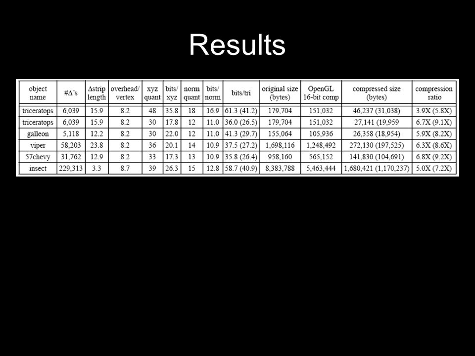
78. Results Software implementation Compression speed: ~3000 triangles / second Decompression speed: ~10,000 triangles / second No information about machine used for evaluation

79. Results

82. Response The technique is supposed to be lossy. –It would be nice to see example images of this. Only one image of an original model is shown. –For the other model examples, there is no original to compare to. Paper claims that compression speed is not important. –Is this true for virtual worlds?

83. Response The technique is supposed to be lossy. –It would be nice to see example images of this. Only one image of an original model is shown. –For the other model examples, there is no original to compare to. Paper claims that compression speed is not important. –Is this true for virtual worlds?

84. Response The technique is supposed to be lossy. –It would be nice to see example images of this. Only one image of an original model is shown. –For the other model examples, there is no original to compare to. Paper claims that compression speed is not important. –Is this true for virtual worlds?

85. Response The technique is supposed to be lossy. –It would be nice to see example images of this. Only one image of an original model is shown. –For the other model examples, there is no original to compare to. Paper claims that compression speed is not important. –Is this true for virtual worlds?

86. Summary First paper on geometry compression Lossy compression of 3D geometry –Reuse vertices in triangle strip using mesh buffer –Shave bits via variable levels of quantization –18-bit indices to reference 48-bit normals –Delta compression saves bits since geometry tends to be local Compressed result is 6 to 10 times fewer bits than original geometry data

87. Summary First paper on geometry compression Lossy compression of 3D geometry –Reuse vertices in triangle strip using mesh buffer –Shave bits via variable levels of quantization –18-bit indices to reference 48-bit normals –Delta compression saves bits since geometry tends to be local Compressed result is 6 to 10 times fewer bits than original geometry data

88. Summary First paper on geometry compression Lossy compression of 3D geometry –Reuse vertices in triangle strip using mesh buffer –Shave bits via variable levels of quantization –18-bit indices to reference 48-bit normals –Delta compression saves bits since geometry tends to be local Compressed result is 6 to 10 times fewer bits than original geometry data

89. Summary First paper on geometry compression Lossy compression of 3D geometry –Reuse vertices in triangle strip using mesh buffer –Shave bits via variable levels of quantization –18-bit indices to reference 48-bit normals –Delta compression saves bits since geometry tends to be local Compressed result is 6 to 10 times fewer bits than original geometry data