1. Climate change in 19-22 centuries in observational and model data Evgeny Volodin, Institute of Numerical Mathematics RAS, Moscow, Russia

2. 1.Model sensitivity to doubling of CO2. 2.Model and observed trends in 19-20 centuries. 3.Future climate scenarios in 21-22 centuries.

3. Model sensitivity to doubling of CO2 is studied on the basis of experiments with: 1.Coupled atmosphere and full ocean general circulation models. Equilibrium response can be achieved in very long runs (about 1000 years) because of deep ocean thermal inertia. Usually transient response is studied. 2.Coupled atmosphere model and 50-m ocean. Model use heat flux adjustment to reproduce observed climate. Equilibrium response can be achieved in 15-20 years.

4. Longwave (full black), shortwave (dashed) and total (red) radiation forcing due to doubling of CO2. Positive means downward.

5. Radiation heating due to doubling of CO2.

6. Radiation forcing due to doubling of CO2 ΔF is about 4 W/m 2. What about near-surface warming ΔT? If we assume that in control climate F=σT 4 and F+ΔF=σ(T+ΔT) 4, than ΔT = 1.1 K 2. If we take into account also positive feedback with water vapour (assuming constant relative humidity), than ΔT = 2.0 K 3. If we take into account also surface albedo feedback, we have ΔT = 2.3 – 2.7 K Real climate models have ΔT = 1.5 – 4.5 K. For some models this parameter can be as large as 8 – 11 K. Main reason of uncertainty is different sensitivity of model cloudiness. In models with low ΔT usually we have low ΔCRF (cloud radiation forcing). In models with high ΔT we have high ΔCRF.

7. Cloud water change (10 -6 kg/kg) due to doubling of CO2 in the model

8. ΔT (K) for transient response to doubling of CO2 (1%/year increase of CO2, years 61-80) in AOGCMs participating in CMIP2. MODEL TLC NCAR-WM GFDL LMD CCC UKMO3 CERF CCSR CSIRO GISS UKMO BMRC ECHAM3 MRI IAP NCAR-CSM PCM INM NRL 3.77 2.06 1.97 1.93 1.86 1.83 1.75 1.73 1.70 1.59 1.54 1.50 1.48 1.26 1.14 0.99 0.75 ? - + - + - +

9. The difference D of surface shortwave radiation in control run between models with high global warming (above 1.69K) and low global warming (below 1.69K) for 18 CMIP models

10. Projection of SW-radiation in control run onto D versus global warming for 18 CMIP models. C=0.73

11. Change of zonal mean temperature (K) due to doubling of CO2 in INM CM3.0. Full ocean, transient response.

12. Response of near-surface air temperature (K) to doubling of CO2. Transient experiment for INM CM3.0.

13. Temperature response to doubling of CO2 in November-April (up) and May-October (down) in INM CM3.0 Precipitation response to doubling of CO2 in November - April (up) and May – October (down) in INM CM3.0

14. Response of SLP to doubling of CO2 in November – April in INM CM3.0 Near-surface air temperature change in November – April induced by change of atmosphere dynamics after doubling of CO2

15. December - February June - August Change of near-surface air temperature at 30E- 130E due to doubling of CO2. Black – all months, Blue – coldest months, Violet – daily minimum in coldest months, Red – warmest months, Dark red – daily maximum in warmest months

16. December - February June - August Relative change of precipitation due to doubling of CO2 in INM CM3.0 averaged over 30E-130E. Black – all months, Blue – the most wet months, Red – the most dry months.

17. Temperature change in the ocean due to doubling of CO2.

19. About 20 models are participating now in comparison of modeling climate of 19-20 century and future climate changes in 21-22 centuries. The results will be used in 4-th IPCC report.

23. Global averaged near-surface air temperature in control run, forcing for 1871 (blue), and run with forcing for 1871-2000 (green)

24. 10-year averaged temperature change in 1871-2000 for the observations (thick) and INM CM3.0 (difference between control run and run with real forcing, thin)

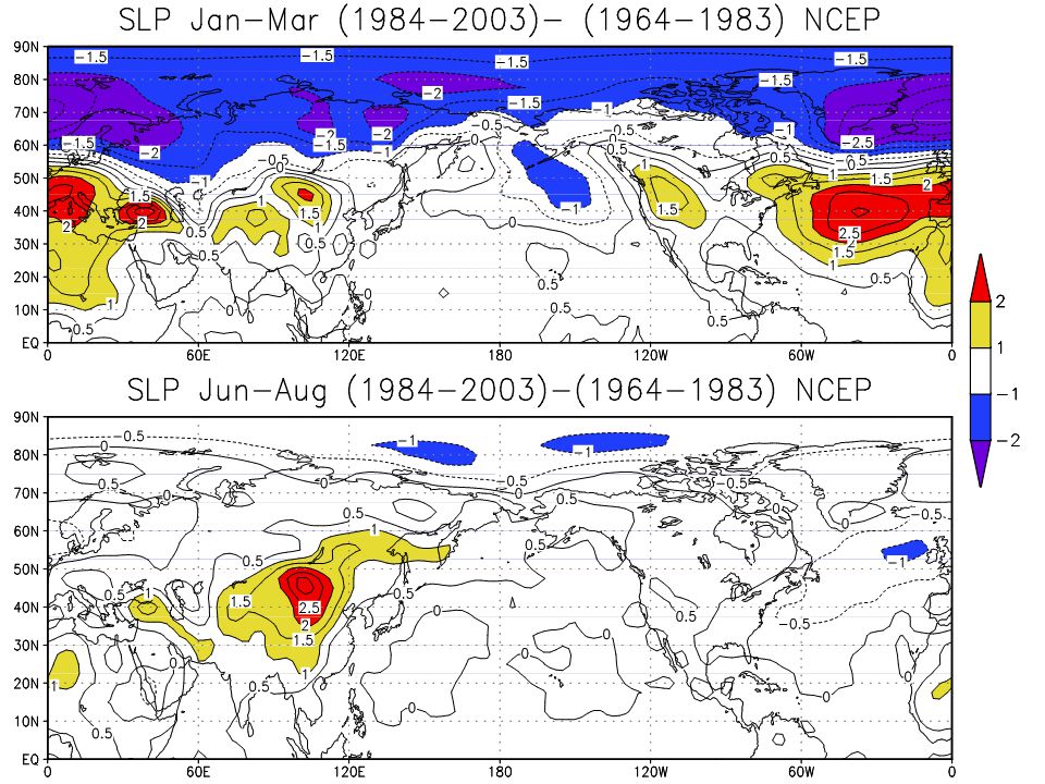
26. Zonal mean temperature from NCEP 1984-2003 minus 1964-1983.

27. Zonal mean temperature in INM CM3.0 1984-2003 minus 1964-1983

31. Month

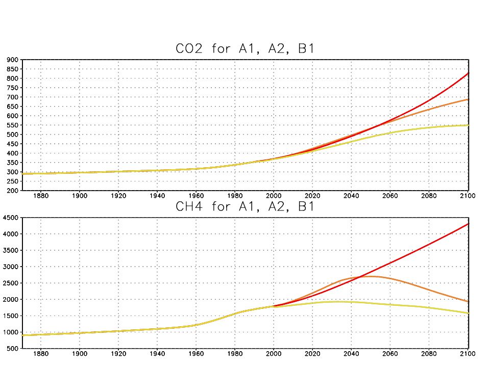
32. Global averaged temperature in control run (blue), run for XX century (green), B1 (yellow), A1B (orange) and A2 (red)

34. Sea ice square in Arctic (top) and Antarctic (bottom) in March (blue) and September (red) in 1871-2200. Data of INM CM3.0, Scenario A1.

36. Sea level change in INM CM3.0 due to thermal enhancement (full) and Antarctic and Greenland ice balance change (dotted). Data of run for XX century and B1 (green), A1B (orange) and A2 (red).