1.  REVIEW  GO OVER HOMEWORK SET #3  CONTINUE CONSUMER BEHAVIOR APPLIED ECONOMICS FOR BUSINESS MANAGEMENT Lecture #3

2. Derivation of the consumer demand function As in the previous example (i.e., changing the price of one commodity and finding the new consumer equilibrium point), if we continue to change, we can get the following:

3. We see that as p 1 changes, ceteris paribus,  shift in the budget line  new consumer equilibrium point

4. Consumer Demand Function Using these consumer equilibrium points, we can derive the consumer’s demand for z 1.

5. Consumer Demand Function Demand illustrates the quantities of a good (commodity) consumer would be willing to purchase at alternative prices, ceteris paribus.

6. Mathematical Derivation of Demand A consumer’s ordinary demand function (called the Marshallian demand function) is derived from utility maximization subject to a budget constraint.

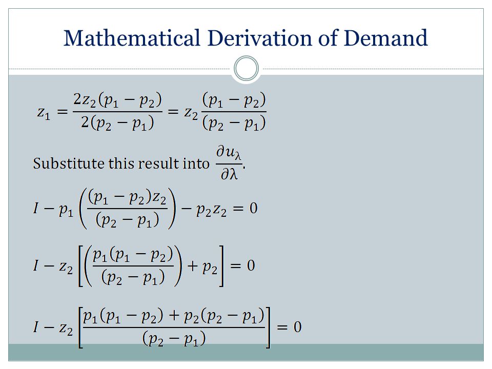
7. Mathematical Derivation of Demand  constrained objective function

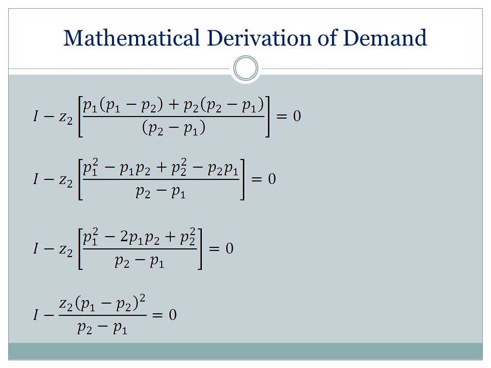
8. Mathematical Derivation of Demand

9. Likewise for z 1, we obtain: Note that these demand functions are a special case since they’re functions of only own price and income. Question: Are these demand functions downward sloping? How can you tell? Downward sloping  the slope is negative

10. Mathematical Derivation of Demand The demand for (Using reciprocals or inverses)

11. Mathematical Derivation of Demand We can easily solve for from the demand function: namely function is negative or demand is downward sloping.

12. Mathematical Derivation of Demand Likewise we get the same result for the consumer demand for z 1 … since negative or demand is downward sloping.

13. So we have the following graph: The law of demand states that price and quantity that are demanded are negatively related.

14. Mathematical Derivation of Demand Is income a positive shifter of demand?

15. In the usual case for demand derived from utility maximization, we have: Mathematical Derivation of Demand

16. To derive this general form, we need to adjust the form of the utility function. Suppose we have: Mathematical Derivation of Demand

21. we can rewrite the equation as:

22. Mathematical Derivation of Demand Demand function is downward sloping: Is income a positive shifter of the demand function?

23. Demand vs. Quantity Demanded Distinction between demand and quantity demanded: [This distinction is usually heavily emphasized in introductory and intermediate microeconomics courses.] Demand refers to the entire schedule. Quantity demanded refers to the quantity purchased by the consumer at a particular price level.

24. Demand Function General form of the demand function: where our usual demand curve. If these other factors change, then demand will shift.

25. Factors Affecting Demand: 1. Changes in income (for normal goods) (vs inferior or Giffen goods)

26. Factors Affecting Demand: 1. Changes in income (for normal goods) 2. Changes in the price of substitutes Take the case of beef and pork (substitutes) If price of pork ↑  demand for beef ↑ Why? Consumers substitute beef for pork when the price of pork ↑ If the price of pork ↓  demand for beef ↓

27. Factors Affecting Demand: 1. Changes in income (for normal goods) 2. Changes in the price of substitutes 3. Changes in the price of complements. Take the case of milk and cereal (complements): If the price of milk ↑  demand for cereal ↓. Why? Milk is an input into cereal consumption. Likewise, if the price of milk ↓  demand for cereal ↑.

28. Factors Affecting Demand: 1. Changes in income (for normal goods) 2. Changes in the price of substitutes 3. Changes in the price of complements. 4. Changes in tastes and preferences.

29. Factors Affecting Demand: 4. Changes in tastes and preferences. No exact relationship, depends on the specific changes. Example: cholesterol scare  demand for eggs ↓. Example: Dietary information about the benefits of fish consumption and the health concerns over red meat consumption  demand for fish ↑  demand for red meats ↓  demand for chicken and turkey ↑

30. Factors Affecting Demand: 1. Changes in income (for normal goods) 2. Changes in the price of substitutes 3. Changes in the price of complements. 4. Changes in tastes and preferences. 5. Increase in population or the number of consumers. Generally, if population ↑  demand for most commodities ↑.

31. Elasticity The concept of elasticity is used as a measure of consumption responsiveness to changes in a particular variable (e.g., own price, income, or cross prices i.e., prices of substitutes or complements).

32. Elasticity We will concentrate on 3 elasticity concepts: own price elasticity of demand income elasticity of demand cross price elasticity of demand We will also evaluate point elasticity rather than arc elasticity.

33. Elasticity Why do economists use elasticity and not slope to measure responsiveness of demand? Because you will get a different measure of responsiveness if you simply change the units of measure on either the vertical or horizontal axis.

34. For example:

35. Now simply change the units of measure of from $/unit to ¢/unit.

36. Elasticity Thus, the slope is not a good measure of responsiveness. Economists prefer using elasticity to measure responsiveness because elasticity is in terms.

37. Elasticity Let the demand for good be: The own price elasticity of demand measures the responsiveness of consumption of good to changes in the price of good, ceteris paribus.

38. Elasticity Why is the own price elasticity negative? To reflect the downward sloping demand schedule.

39. Elasticity the elastic portion of the demand function. the unitary elastic point on the demand function. the inelastic portion of the demand function.

40. Elasticity

41. Example: Estimate the own price elasticity of demand at the point (this point lies on the elastic portion of the demand function)

42. Example: Suppose now you wanted to determine the price elasticity at (this point lies on the inelastic portion of the demand function)

43. Factors affecting the price elasticity of demand: 1.Availability of substitutes (and closeness of substitutes). More substitutes and closer substitutes  more elastic demand.

44. Factors affecting the price elasticity of demand: 1.Availability of substitutes (and closeness of substitutes). 2. Uses of the product. More uses of the product or goods  more elastic demand.

45. Factors affecting the price elasticity of demand: 1.Availability of substitutes (and closeness of substitutes). 2. Uses of the product. 3. Share in consumer budgets. Commodities with larger shares tend to be more elastic. Pencils are a small portion of consumers’ budgets, so if the price of pencils changes, one would not expect a large quantity response. However, items such as automobiles, appliances, etc. tend to be more elastic.

46. Factors affecting the price elasticity of demand: 1.Availability of substitutes (and closeness of substitutes). 2. Uses of the product. 3. Share in consumer budgets. 4. Luxuries vs. necessities

47. Factors affecting the price elasticity of demand: Demand for necessities tend to be more inelastic than luxuries. Demand for gasoline, milk, salt, etc. tend to be inelastic. Demand for large screen TVs, vacations abroad, etc. tend to be elastic. 4. Luxuries vs. necessities

48. Factors affecting the price elasticity of demand: 1.Availability of substitutes (and closeness of substitutes). 2. Uses of the product. 3. Share in consumer budgets. 4. Luxuries vs. necessities 5. Time period for consumption.

49. Factors affecting the price elasticity of demand: 5. Time period for consumption. Over a long period of time, consumers can either adjust their budgets to a price change in a particular commodity or find substitutes. Consequently, the long run elasticity tends to be more elastic than the short run price elasticity.

50. Examples: Gasoline -0.40 -1.50 Housing -0.30 -1.88

51. Other Elasticities: a. Income elasticity The income elasticity measures the responsiveness of good to changes in income, ceteris paribus.

52. Plotting and (income), one traces out the Engel curve.

53. Other Elasticities: a. Income elasticity b. Cross price elasticity The cross price elasticity of demand measures the responsiveness of to changes in the price of other goods ceteris paribus.

54. Cross Price Elasticity  consumers switch to z, so the demand for z ↑

55. Cross Price Elasticity As ↑  quantity demanded of ↓ Since and are complements,  demand for ↓

56. Relationship Among Elasticities There are 3 key relationships among elasticities: homogeneity condition Slutsky or symmetry condition Engel condition The theory behind these elasticity relationships makes a certain assumption regarding individual consumer behavior.

57. Elasticity Matrix Given n goods and income, we have the following elasticity matrix:

58. Elasticity Matrix Own price elasticities are located on the diagonal. Cross price elasticities are on the off-diagonal. Income elasticities are on the last column.

59. Homogeneity condition The homogeneity condition states that the sum of the own and cross price elasticities and income elasticities for a particular commodity is zero.

60. Homogeneity condition The homogeneity condition stems from Euler’s Theorem which states that if a function is homogeneous of degree k then If then the function is homogeneous of degree zero (HD0).

61. Since, we can rewrite this as: Homogeneity condition Now divide through by : This is the homogeneity condition.

62. Homogeneity condition The meaning of the homogeneity condition is that the magnitude of the own price elasticity must be consistent with the cross price elasticities and income elasticity of that commodity.

63. Example Demand for beef: Own price elasticity -0.62 Cross price with pork 0.11 Cross price with lamb 0.01 Cross price with chicken 0.06 All other cross elasticities -0.01 Income elasticity 0.45 ∑ = 0

64. Slutsky or Symmetry Condition This condition specifies a specific relationship between and The Hotelling-Jureen relationship states:

65. Hotelling-Jureen

66. Engel Condition The consumer’s budget can be written as:  assuming all income is spent on commodities The effects of changes in income on consumption can be obtained by differentiating the above equation with respect to I :

67. Engel Condition Multiply each component by

68. Engel Condition Recall that: and This states that the weighted sum of the income elasticities for all items in the consumer’s budget should sum to 1.

69. Market Demand Conditions How are market demand functions obtained from consumer demand functions? Quantities demanded or purchased by consumers are added together for each price level.

70. Market Demand Conditions

71. Consumer #1 Consumer #2 Consumer #3

72. Market Demand Conditions