1. Chapter 3 Economic Order Quantity

2. Defining the economic order quantity

3. Background to the model The approach is to build a model of an idealized inventory system and calculate the fixed order quantity that minimizes total costs. This optimal order size is called the economic order quantity (EOQ).

5. Assumption for a basic model The demand is known exactly, is continuous and is constant over time. All costs are known exactly and do not vary. No shortages are allowed. Lead time is zero – so a delivery is made as soon as the order is placed.

6. Other assumptions implicitly in the model We can consider a single item in isolation, so we cannot save money by substituting other items or grouping several items into a single order. Purchase price and reorder costs do not vary with the quantity ordered. A single delivery is made for each order. Replenishment is instantaneous, so that all of an order arrives in stock at the same time and can be used immediately.

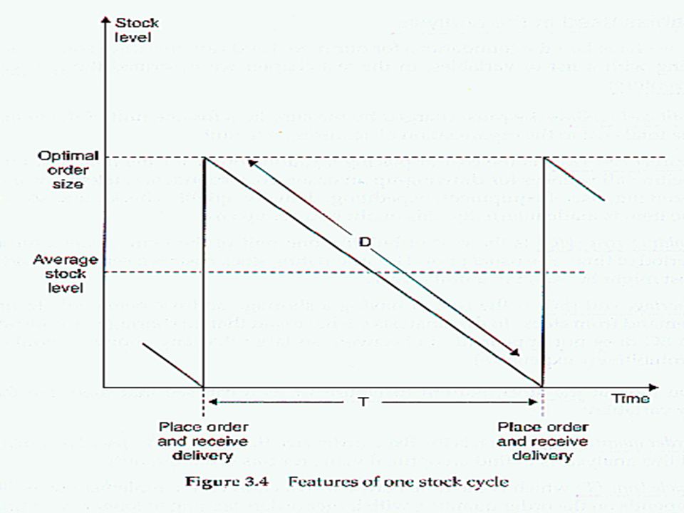
7. The most important assumption here is that demand is known exactly, is continuous and constant over time (Fig. 3.2) The assumptions give an idealized pattern for a stock level. (Fig. 3.3)

9. Variables used in the analysis Four costs of inventory 1.Unit cost (UC) 2.Reorder cost (RC) 3.Holding cost (HC) 4.Shortage cost (SC)

10. Three other variables: Order quantity (Q) Cycle time (T) Demand (D)

11. Derivation of the economic order quantity Three steps: 1.Find the total cost of one stock cycle. 2.Divided this total cost by the cycle length to get a cost per unit time. 3.Minimize this cost per unit time.

13. Amount entering stock in cycle = amount leaving stock in cycle So Q = D x T Total cost per cycle = unit cost + reorder cost + holding cost (component)

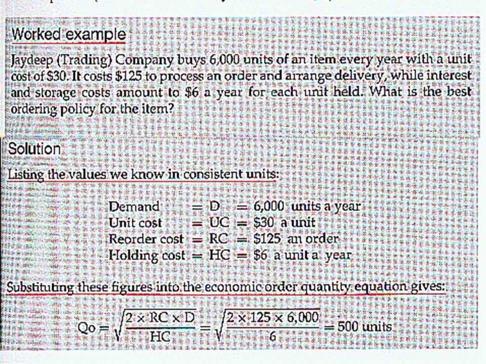
20. The optimal time between orders is: To = Qo/D =500/6,000 = 0.083 years = 1 month The associate variable cost is: VCo = HC × Qo = 6 × 500 = $3,000 a year This gives a total cost of: TCo = UC × D + VCo = 30 × 60000 + 3000 = $183,000 a year

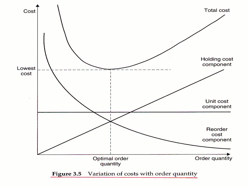
24. Summary We have built a model of an idealized inventory system that relates order size to costs and demand. This shows that large, infrequent orders have a high holding cost component, so the total cost is high: small, frequent orders have a high reorder cost component, so the total cost is also high. A compromise finds the optimal order size – or economic order quantity – that minimizes inventory costs.

25. Adjusting the economic order quantity Moving away from the EOQ The EOQ suggests fractional value for things which come in discrete units (e.g. an order for 2.7 lorries) Suppliers are unwilling to split standard package sizes. Deliveries are made by vehicles with fixed capacities. It is simply more convenient to round order sizes to a convenient number.

26. How much costs would rise if we do not use the EOQ Example: D = 6000 units a year Unit cost, UC = £30 a unit Reorder cost, RC = £125 an order Holding cost, HC = £7 a unit a year

34. Order for discrete items This suggests a procedure for checking whether it is better to round up or round down discrete order quantities: 1.Calculate the EOQ, Qo. 2.Find the integers Q’ and Q’-1 that surround Qo. 3.If Q’×(Q’-1) is less than or equal to Qo 2, order Q’. 4.If Q’×(Q’-1) is greater than Qo 2, order Q’-1.

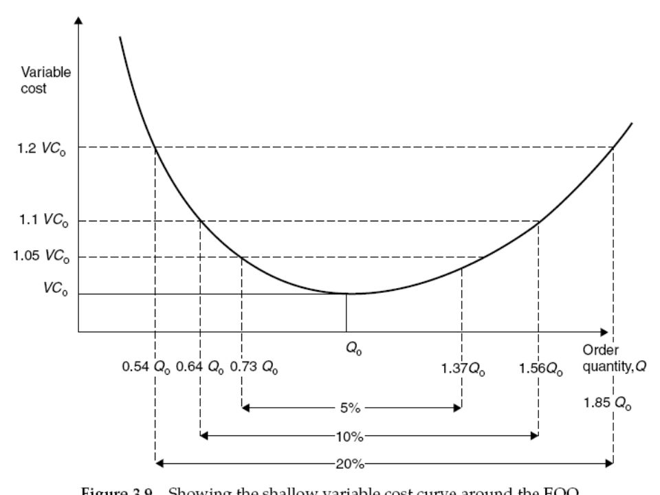
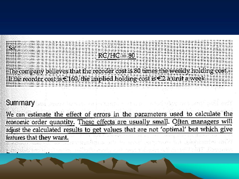
37. Uncertainty in demand and costs Error in parameters Few organizations know exactly what demand they have to meet in the future. The variable cost is stable around the EOQ and small errors and approximations generally make little difference.

41. Adjusting the order quantity

42. or

46. Adding a finite lead time Time for order preparation Time to get the order to the right place in suppliers Time at the supplier Time to get materials delivered from suppliers Time to process the delivery

47. Reorder level The amount of stock needed to cover the lead time is also constant at: Lead time × demand per unit time Reorder level = lead time demand = lead time × demand per unit time ROL = LT × D

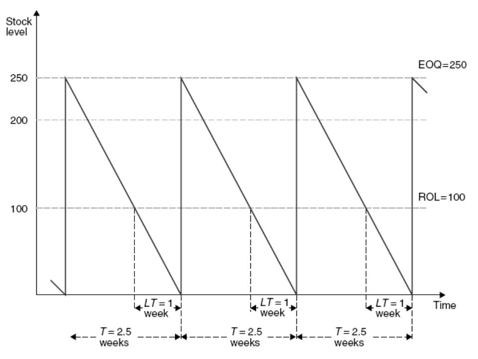
50. (b) Substituting value LT = 2 and D = 100, gives ROL = LT × D = 2 × 100 = 200 units As soon as the stock level declines to 200 units, Carl should place an order for 250 units.

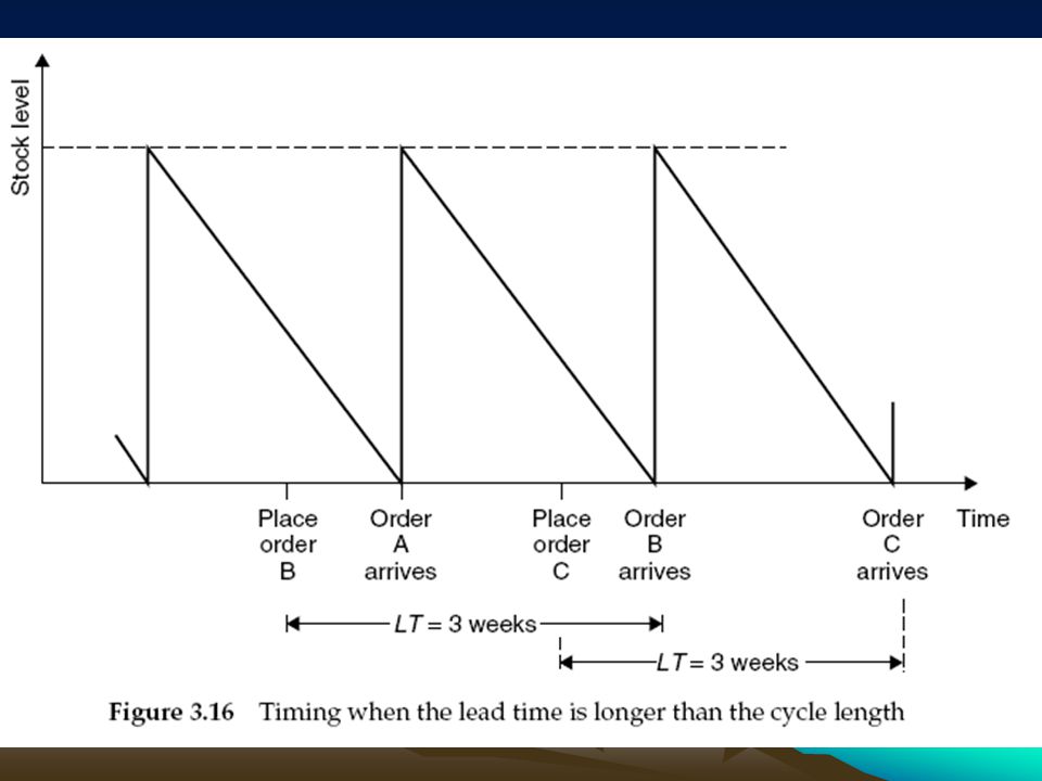
52. Longer lead times The cycle length is: T = Q/D = 250/100 = 2.5 weeks What happens when the lead time is increased to 3 weeks ? ROL = LT × D = 3 × 100 = 300

53. Stock on hand + stock on order = LT × D =300 units Reorder level = lead time demand – stock on order n × T < LT < (n+1) × T Reorder level = lead time demand – stock on order ROL = LT × D – n × Qo

56. Some practical points This chapter has shown when to place an order – set by the reorder level. How much to order – set by the economic order quantity. A two-bin system gives a simple procedure for controlling stock without computers or continuous monitoring of stock levels.

57. Three-bin system The two-bin system can be extended to a three-bin system which allows for some uncertainty. The third bin holds a reserve that is only used in an emergency. The normal stock is used from bin A.

58. Our calculations assume that the lead time is known exactly and constant. In practice, there can be quite wide variation, allowing for availability, supplier reliability, checks on deliveries, transport conditions, customs clearance, delays in administration, and so on.

59. Some stock levels are not recorded continuously but are checked periodically, perhaps at the end of the week. Then an unexpectedly large demand might reduce stocks well below the reorder level before they are checked.

60. Another problem appears with large stocks, such as chemical tanks, coal tips or raw materials, where the stock level is only known approximately. Then the reorder level might be passed without anyone noticing.

61. We have assumed that the order size is independent of the lead time and the reorder level. In practice, people often prefer larger orders if there are longer lead times, and they raise the reorder level to add an element of safety. The reorder level can be also influence the order size, with people typically placing smaller orders with higher reorder levels.