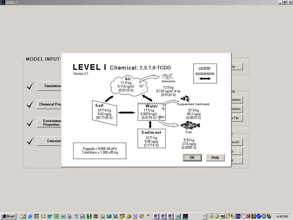
2. Fugacity Models Level 1 : Equilibrium
Level 2 : Equilibrium between compartments & Steady-state over entire environment
Level 3 : Steady-State between compartments
Level 4 : No steady-state or equilibrium / time dependent

3. “Chemical properties control”
Level 1 : Equilibrium
“Chemical properties control”
fugacity of chemical in medium 1 =
fugacity of chemical in medium 2 =
fugacity of chemical in medium 3 =
…..

4. Mass Balance Total Mass = Sum (Ci.Vi) Total Mass = Sum (fi.Zi.Vi)
At Equilibrium : fi are equal
Total Mass = M = f.Sum(Zi.Vi)
f = M/Sum (Zi.Vi)

6. Fugacity Models Level 1 : Equilibrium
Level 2 : Equilibrium between compartments & Steady-state over entire environment
Level 3 : Steady-State between compartments
Level 4 : No steady-state or equilibrium / time dependent

7. fugacity of chemical in medium 1 = fugacity of chemical in medium 2 =
Level 2 :
Steady-state over the entire environment & Equilibrium between compartment
Flux in = Flux out
fugacity of chemical in medium 1 =
fugacity of chemical in medium 2 =
fugacity of chemical in medium 3 =
…..

8. Level II fugacity Model:
Steady-state over the ENTIRE environment
Flux in = Flux out
E + GA.CBA + GW.CBW = GA.CA + GW.CW
All Inputs = GA.CA + GW.CW
All Inputs = GA.fA .ZA + GW.fW .ZW
Assume equilibrium between media : fA= fW
All Inputs = (GA.ZA + GW.ZW) .f
f = All Inputs / (GA.ZA + GW.ZW)
f = All Inputs / Sum (all D values)

10. Fugacity Models Level 1 : Equilibrium
Level 2 : Equilibrium between compartments & Steady-state over entire environment
Level 3 : Steady-State between compartments
Level 4 : No steady-state or equilibrium / time dependent

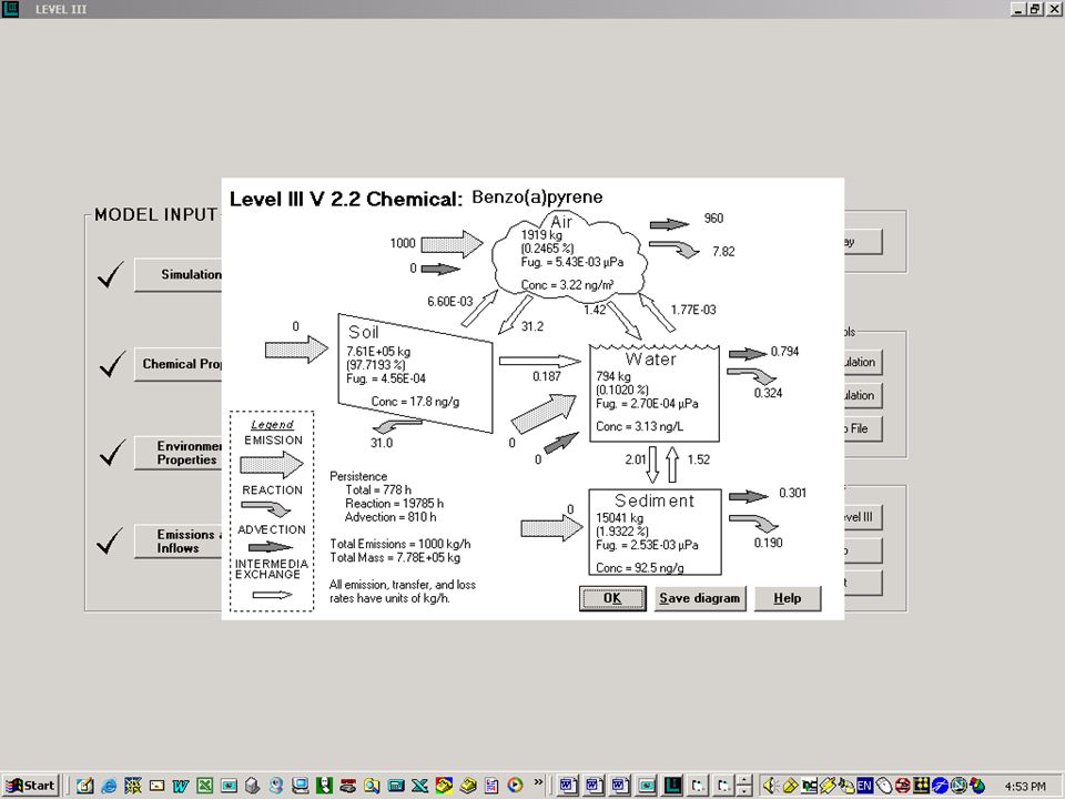
11. Level III fugacity Model:
Steady-state in each compartment of the environment
Flux in = Flux out
Ei + Sum(Gi.CBi) + Sum(Dji.fj)= Sum(DRi + DAi + Dij.)fi
For each compartment, there is one equation & one unknown.
This set of equations can be solved by substitution and elimination, but this is quite a chore.
Use Computer

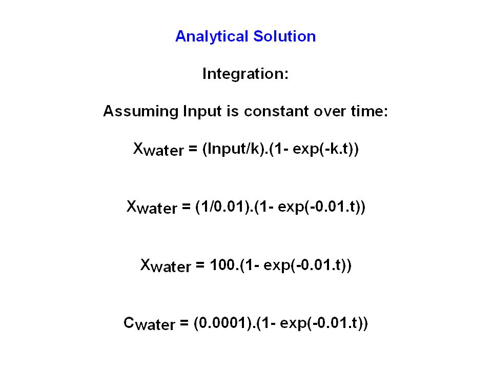
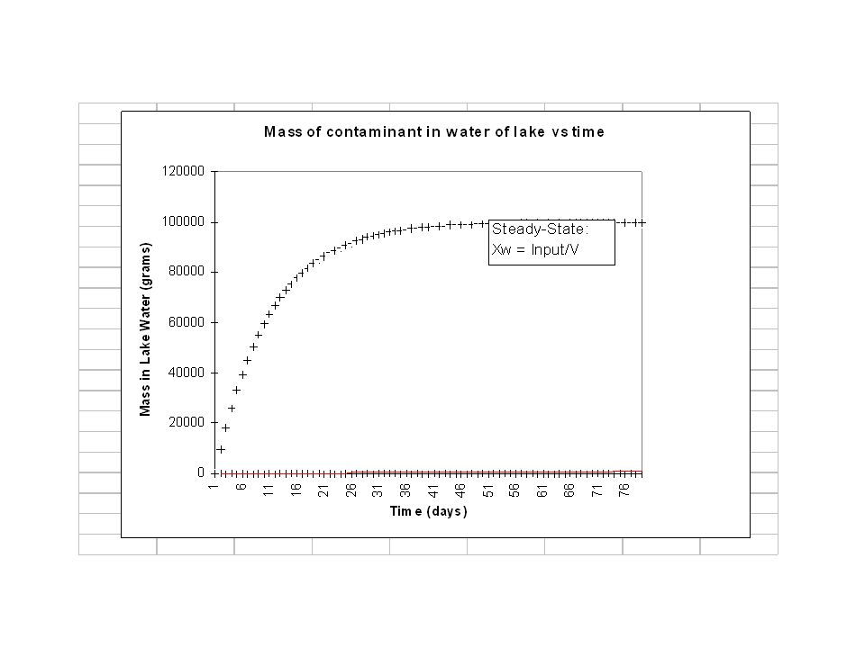
13. Time Dependent Fate Models / Level IV

22. Evaluative Models vs. Real Models

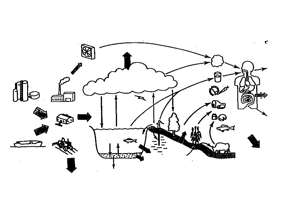
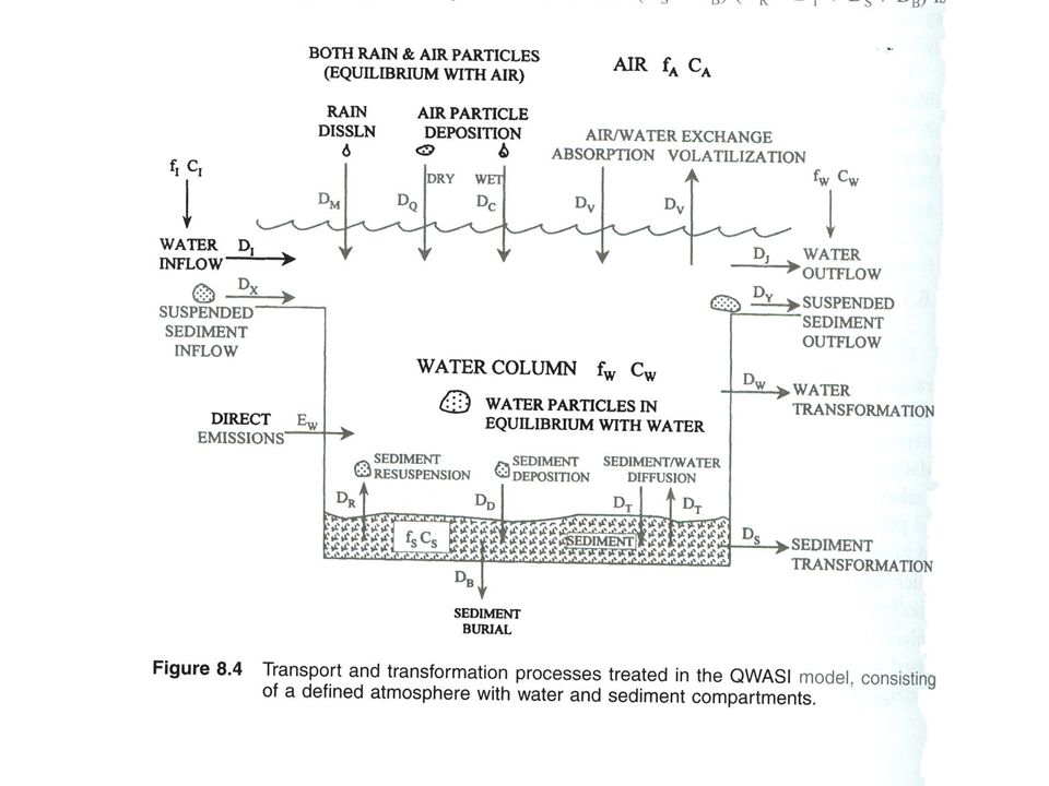
23. Recipe for developing mass balance equations
1. Identify # of compartments
2. Identify relevant transport and transformation processes
3. It helps to make a conceptual diagram with arrows representing the relevant transport and transformation processes
4. Set up the differential equation for each compartment
5. Solve the differential equation(s) by assuming steady-state, i.e. Net flux is 0, dC/dt or df/dt is 0.
6. If steady-state does not apply, solve by numerical simulation

26. Application of the Models
To assess concentrations in the environment
(if selecting appropriate environmental conditions)
To assess chemical persistence in the environment
To determine an environmental distribution profile
To assess changes in concentrations over time.

27. What is the difference between
Equilibrium & Steady-State?

28. Time Dependent Fate Models / Level IV