1. Dan Rawding, Thomas Buehrens, and Charlie Cochran

2. OUTLINE Goals & Notes Hierarchical Models Wind River Steelhead Background CJS Model, Tagging Sites, Recovery Sites Model Selection & GOF Test Results Management Implications Summary

3. GOALS & NOTES Use tag data from Wind River steelhead parr, smolt, and adult PIT tagging to estimate life stage survival and capture probabilities using Cormack-Jolly-Seber (CJS) model In CJS model survival (φ)= apparent survival, which is survival in the study area. In this case, if we PIT tagged resident 0. mykiss parr that do not emigrate as smolts survival estimates are biased low.

4. Wind River Steelhead Located at RM 153 ~ 11 mile upstream BON Wild steelhead sanctuary since 2000 Escapement (range 200-1500);mean (600+) Summer steelhead - 95% to 99% of escapement Freshwater Age - age 2 ~75% & age 3 ~ 25% Marine Age- age 1<5%, age 2~85%, age 3<10% Annual (2.2s) and Skip Repeat Spawners (2.2s1) PIT Tagging smolts since 2003 annual tag range (1100-2500), parr since 2007 tag annual range (300-600), & adults since 2008 annual tag range (30-300)

5. CJS Model This CJS model is life cycle model using tagging, detection, and recapture sites to partition life stage survival. Buchanan and Skalski (2007) developed a life cycle model to estimate smolt survival of spring Chinook from LWG to BON and adult returns to LWG. Extended the above model to include: parr to smolt survival, repeat spawners, Applied statistical approaches (e.g. random effects) to develop estimates for small populations Assume all parr tagged in spring emigrate as smolts following year. Most fish are PIT tagged at the smolt stage & CJS model tracks smolt outmigration cohorts Adults tagged at Shipherd Falls ladder added to appropriate smolt outmigration year based on scale ages.

7. Wind River Steelhead Life Cycle White – detection site Grey-tagging/recapture site

8. CJS Wind River m-array Node LW_STBONsmTWX/ESBONmaSFTmaBONk1TWXk1BONr1 Not Seen UR_ST10430000299 LW_ST0187145640000761 BONsm0034150000138 TWX/ES0003000024 BONma00001051267 SFTma0000045117211 BONk10000000941 TWXk1000000002 BONr10000000016 Create individual capture histories (0,1) at each site based on PTAGIS query Sum individual capture histories to create m-array for analysis

9. Data Analysis Pooled/Constant (all survivals and/or capture prob. are equal at each life stage or site) Independent/Individual (all survivals and/or capture prob. are independent at each life stage or site) Random Effects/Hierarchical/Multi-level All annual adult PIT tag detection efficiencies at BON come from a common distribution of detection efficiencies and their ordering does not affect the model (exchangeable) Individual estimates from hierarchical models borrow strength from other annual detection efficiencies because they are similar; reduces model overfitting; hierarchical models are a compromise between independent and fully pooled estimates. Hierarchical parameter estimates have improved precision because they shrink toward the mean; shinkage depends on the variance of the random parameters. Borrowing strength is often viewed as being beneficial when data is sparse, as in many survival and abundance studies.

10. Model Selection Deviance Information Criteria (DIC), a Bayesian analog for AIC that can be used to evaluate hierarchical models, was used for model selection (lower values provide better fit). Models 9 smolt cohorts (2003-11). Eight survival estimates per cohort (survival from parr through repeat spawners to BON) Seven capture estimates per cohort (Wind River smolt trap to repeat spawners at BON) Evaluated nine models combining hierarchical/random effects, pooled, and independent for capture and survival

11. Model Selection & GOF Test Model (p, phi)Deviance Parameters DICΔDIC Bayesian P-value Median P-value RE,RE662.1685.46747.620.07 – 0.680.42 RE, Ind670.4494.96765.4017.780.07 – 0.790.30 Ind, RE676.587111.03787.6240.000.10 – 0.550.25 Ind, Ind678.71127.27805.9858.360.16 – 0.710.26 Ind, Pool812.5487.38899.92152.300.00 – 0.180.04 RE,Pool823.114157.99981.11233.490.00 – 0.200.02 Pool, Ind914.0368.04982.07234.450.00 – 0.350.00 Pool,RE935.41379.181014.59266.970.00 – 0.200.00 Pool, Pool1757.9015.931773.821026.200.00 – 0.000.00 ΔDIC values < 10 little model support Bayesian P-values 0.5 perfect fit (0.025-0.975) acceptable fit Model 1 - with Random effects for survival has greatest support

14. CJS Assumptions Every marked fish present at sampling period i has the same prob. of capture (p). Every marked animal present at sampling period i has the same prob. of survival (φ) to the next period. – Based on omnibus Bayesian GOF test ( P-values [0.07-0.68], median = 0.42) assumption is met. Similar GOF tests in the program MARK. Marks are not lost/overlooked and correctly reported. – Short-term tag loss in Wind parr and smolt from double tagging experiments ~1%. – Knudsen et al. (2009) identified tag loss and mortality (2% juveniles & 18% adults) with PIT tags for hatchery spring Chinook salmon; so our survival estimates are likely biased low through adult stage at BON if Knudsen results are applicable to steelhead.

15. CJS Assumptions Sampling is instantaneous and all fish are released immediately after capture. – Spatial model so tagging or detection site is short compared to distance between sites – Simulations by Hargrove and Borlund (1994) suggests parameters not too sensitive to the instantaneous sampling assumption. The fate of each fish with respect to capture and survival probability is independent of the fate of other fish. – If this assumption not met this leads to overdispersion; estimates will be unbiased but variance will be underestimated.

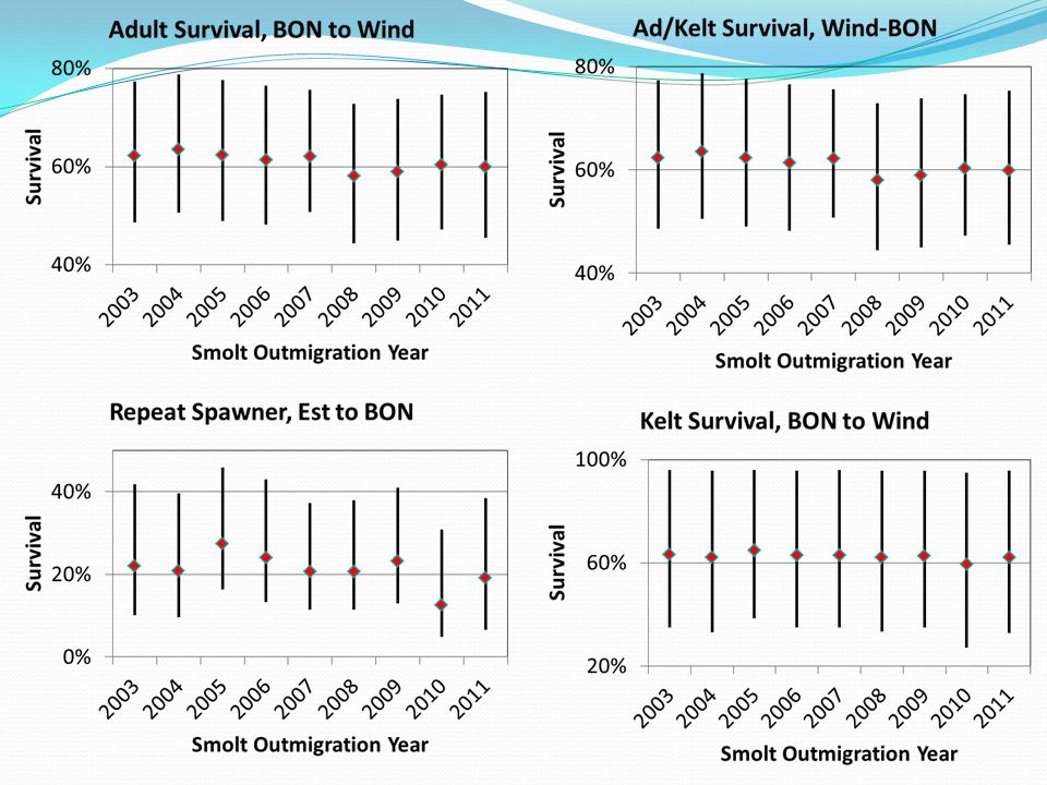
16. Management Implications Wind River SAR were the most variable survival parameter we measured Wind River SAR had highest correlation with total cohort survival (0.88). Correlation between total survival and BON-Est survival had second highest correlation (0.85)

17. Management Implications Few Wind steelhead detections at other PIT sites ~37% of the Wind River steelhead do not survive the 13 miles (BON to SF). Wind River PIT tag Z6 fall harvest rate~ 7% in 2010 & ~12% in 2011 Harvest rates are unknown in other Z6 fisheries and recreational wild release fisheries. BON pool can be in excess of 22 degrees, which exceeds the 1 & 7-day average maximum of 22 & 17 degrees

18. Management Implications Apparent survival for parr to smolt is ~ 10% for primary rearing area between upper and lower traps. No parr tagging from 2003 to 2007, so the estimate is the hierarchical estimate. Density dependence & parr residualization may contribute to the low survival for this life stage.

19. Management Implications Approximately 17% (range 5% to 30%) of the kelts are detected at BON; most are detected in the corner collector or ice and trash sluiceway. Approximately 20% of the kelts (range 13% to 27%) survive from entry into the estuary as kelts to returning adults (repeats) at BON.

20. Columbia R. Kelt Survival Rates Repeat Kelt to Adult Kelt TagRecovery Return (KAR)Location Reference 1%LWGBONKeefer et al. 2008 6%MCNBONKeefer et al. 2008 6%JDABONKeefer et al. 2008 14%BON This presentation Travel Time of Kelts from Radio Tracking Studies – 43-54 km/day-Skeena – 100 km/day - Frazier – 99-111 km/day –Columbia @Hanford Reach – 13-16 km/day – Snake (Impounded) – 39 km/day – Upper Columbia (Impounded)

21. Management Summary Unaccounted for loss of adult steelhead is >20% between BON and Wind. If loss was reduced to zero, the population in the Wind would immediately increase >35% Likely mortality sources include natural mortality, increased mortality due to temperature in BON, and unaccounted fishery mortality Odds of a Wind River kelt surviving to a repeat spawner are 2.5 to 14 times higher than those reported by Keefer et al. 2008. Delay in travel time is likely due to difficulty in kelts locating passage routes at dams, impoundments delaying travel time, and reduced spring freshet due to water storage. Delayed travel time of kelts leads to later ocean entry, which may not be synchronized with ocean food supply and environmental conditions that lead to high survival.

22. Summary CJS model is typically applied to in the Columbia River to estimate juvenile reach survival but can be used to estimate survival/mortality by life stage for anadromous fish. This approach allows an estimate of survival by life stages/migration periods to identify limiting stages. I have only discussed a fraction of the life cycle information available. When few tags are releases or when detection rates are low, hierarchical models can improved the precision of estimates given the assumption of exchangability. Hierarchical approach is not limited to one population between years but could include multiple populations with same year or other approaches.

23. Acknowledgements Bryce Glaser (WDFW) – project management. Rich Zabel (NOAA) - Sand Island and Estuary Trawl photos. Steve VanderPloeg (WDFW) – map. Mary Todd Haight (BPA) for support of Wind River Steelhead monitoring project. Various WDFW, USFS, and USGS technicians for adult and juvenile data collection and PIT tagging.