1. Group 2 Bhadouria, Arjun Singh Glave, Theodore Dean Han, Zhe
Chapter 5. Laplace Transform
Chapter Wave Equation

2. Laplace Transform
Chapter 5

3. 5. Laplace Transform 5.1. Introduction & Definition
5.2. Calculation of the Transform
5.3. Properties of the Transform
5.4. Application to the Solution of Differential Equations
5.5. Discontinuous Forcing Functions; Heaviside Step Function
5.6. Impulsive Forcing Functions; Dirac Impulse Function
5.7. Additional Properties

4. 5.1. Introduction & Definition
The Laplace transform is a widely used integral transform. Denoted , it is a linear operator of a function f(t) with a real argument t (t ≥ 0) that transforms it to a function F(s) with a complex argument s. The Laplace transform has the useful property that many relationships and operations over the originals f(t) correspond to simpler relationships and operations over the images F(s). The Laplace transform has many important applications throughout the sciences.
The Laplace transform is used for solving differential and integral equations. In physics and engineering, it is used for analysis of linear time-invariant systems. In this analysis, the Laplace transform is often interpreted as a transformation from the time-domain, in which inputs and outputs are functions of time, to the frequency-domain, where the same inputs and outputs are functions of complex angular frequency, in radians per unit time. Given a simple mathematical or functional description of an input or output to a system, the Laplace transform provides an alternative functional description that often simplifies the process of analyzing the behavior of the system, or in synthesizing a new system based on a set of specifications.

5. Basic idea

6. Given a known function K(t,s), an integral transform of a function f is a relation of the form
The Laplace Transform of f is defined as
where the kernel function is K(s,t) = e-st , a=0, b= .
F (s) is the symbol for the Laplace transform,
L is the Laplace transform operator,
and f(t) is some function of time, t.

7. How to solve problems Frequency Domain Time Domain Laplace transform
Solve algebraic equation
Inverse Laplace transform
Douglas Wilhelm Harder, University of Waterloo.

8. 5.2. Calculation of the Transform
Since the Laplace Transform is defined by an improper integral, thus it must be checked whether the transform F(s) of a given function f(t) exists, that is
whether the integral converges.

9. EXAMPLE 2.1. Consider the following improper integral.
We can evaluate this integral as follows:
Note that if s = 0, then est = 1. Thus the following two cases hold:

10. EXAMPLE 2.2. Consider the following improper integral.
We can evaluate this integral using integration by parts:
Since this limit diverges, so does the original integral.

11. Exponential order
Suppose that f is a function for which the following hold:
(1) f is piecewise continuous on [0, b] for all b > 0.
(2) | f(t) |  Kect when t  T, for constants c, K, M, with K, M > 0.
A function f that satisfies the conditions specified above is said to to have exponential order as t  
EXAMPLE 2.3. Is f(t)=exp(4t)cost of exponential order?
Solution: Yes.
Therefore, K=10, c=4, and T=10 for instance
EXAMPLE 2.4. Is f(t)=ln(t) of exponential order?
Solution: Yes.
Therefore, K=100, c=1, and T=10 for instance

12. Piecewise Continuous
If an interval [a, b] can be partitioned by a finite number of points a = t0 < t1 < … < tn = b such that Then the function f is piecewise continuous Or we can say f is piecewise continuous on [a, b] if it is continuous there except for a finite number of jump discontinuities.
Picture from Paul's Online Math Notes

13. EXAMPLE 2.5. Piecewise continuous function
Consider the following piecewise-defined function f.
(a)
From this definition of f, and from the graph of f below, we see that f is piecewise continuous on [0, 3].
(b)
From this definition of f, and from the graph of f below, we see that f is
NOT piecewise continuous on [0, 3].

14. THEOREM 2.1 Existence of the Laplace Transform
Let f(t) satisfy these conditions:
f(t) is piecewise continuous on for every A>0,
f(t) is of exponential order as
That is to say
(1) f is piecewise continuous on [0, b] for all b > 0.
(2) | f(t) |  Kect when t  T, for constants c, K, M, with K, M > 0.
Then the Laplace Transform of f exists for s > c.

15. Inverse Laplace transform operator
By definition, the inverse Laplace transform operator,
L-1, converts an s-domain function back to the corresponding time domain function:
Importantly, both L and L-1 are linear operators.
Thus,

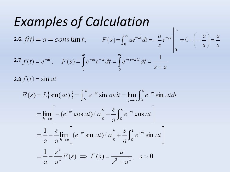
16. Examples of Calculation
2.6.
2.7
2.8

17. Laplace transform table

18. 5.3. Properties of the Transform
A various types of problems that can be treated with the Laplace transform include ordinary and partial differential equations as well as integral equations.
THEOREM 3.0
The transform of an expression that is multiplied by a constant is the constant multiplied by the transform. That is:

19. THEOREM 3.1 Linearity of the Transform
Suppose u and v are functions whose Laplace transforms exist for s > a1 and s > a2, respectively.
Then, for s greater than the maximum of a1 and a2, the Laplace transform of au(t) + bv(t) exists. That is,
With
Therefore

20. f (t) = 5e-2t - 3sin(4t) for t  0.
EXAMPLE 3.1.
f (t) = 5e-2t - 3sin(4t) for t  0.
by linearity of the Laplace transform, and using results of Laplace transform table, the Laplace transform F(s) of f is:

21. THEOREM 3.2 Linearity of the Inverse Transform
For any U(s) and V(s) such that the inverse transforms
For any constants a,b.
Basic idea :
Consider a general expression,
Expand a complex expression for F(s) into simpler terms, each of which appears in the Laplace Transform table. Then you can take the L-1 of both sides of the equation to obtain f(t).

22. EXAMPLE 3.2. Perform a partial fraction expansion (PFE)
where coefficients and have to be determined.
To find : Multiply both sides by s + 1 and let s = -1
To find : Multiply both sides by s + 4 and let s = -4
Therefore,

23. THEOREM 3.3 Transform of the Derivative
Let f(t) be continuous and f’(t) be piecewise continuous on 0≤t≤t。For every finite t。, and let f(t) be of exponential order as t   so that there are constants K, c, T such that | f(t) |  Kect when t  T. Then L{f’(t)} exists for all s>c.
This is a very important transform because derivatives appear in the ODEs we wish to solve.
Similarly, for higher order derivatives:
where:

24. Proof
Deriving the Laplace transform of f (t ) often requires integration by parts. However, this process can sometimes be avoided if the transform of the derivative is known:
For example, if f (t ) = t then f ‘ (t ) = 1 and f (0) = 0 so that, since:
That is:
It has already been established that if:
then:
Now let
so that:
Therefore:

25. EXAMPLE 3.3 For example, if: then: and Similarly:
And so the pattern continues.
EXAMPLE 3.3
Then substituting in:
yields
So:

26. COMMENT: Difference in
EXAMPLE 3.4
*Additional Section
COMMENT: Difference in
The values are only different if f(t) is not continuous at t=0
Example of discontinuous function: u(t)

27. EXAMPLE 3.5 Try to solve the differential equation:
take the Laplace transform of both sides of the differential equation to yield:
Resulting in:
The right-hand side can be separated into its partial fractions to give:
From the table of transforms it is then seen that:
Thus,

28. THEOREM 3.4 Laplace Convolution Theorem
If both exist for s>c, then
As Laplace convolution of f and g.

29. Proof:
We have,
therefore

30. EXAMPLE 3.6 EXAMPLE 3.7 If f(t)=exp(t), g(t)=t, then
Schiff. Joel L. The Laplace transform: theory and applications. P92

31. 5.4. Application to the Solution of Differential Equations
Laplace transforms play a key role in important engineering concepts and techniques.
Examples:
Transfer functions
Frequency response
Control system design
Stability analysis …

32. Solution of ODEs by Laplace Transforms
Procedure:
Take the L of both sides of the ODE.
Rearrange the resulting algebraic equation in the s domain to solve for the L of the output variable, e.g., F(s).
Perform a partial fraction expansion.
Use the L-1 to find f(t) from the expression for F(s).

33. EXAMPLE 4.1. Solve Equation with initial conditions
Laplace transform is linear
Apply derivative formula
Rearrange
Take the inverse

34. EXAMPLE 4.2.
resulted in the expression
Take L-1 of both sides:

35. EXAMPLE 4.3.
Taking Laplace transforms of both sides of this equation gives:
K.A. Stroud. Engineering Mathematics. P1107

36. EXAMPLE 4.4.
A mass m is suspended from the end of a vertical spring of constant k (force required to produce unit stretch). An external force f(t) acts on the mass as well as a resistive force proportional to the instantaneous velocity. Assuming that x is the displacement of the mass at time t and that the mass starts from rest at x=0,
Set up a differential equation for the motion
Find x at any time t
Solution:
(a)The resistive force is given by –βdx/dt. The restoring force is given by –kx. Then by Newton’s law,

37. EXAMPLE 4.4.
(b) Taking the Laplace transform of (1), using we obtain So that on using (2) Where There are three cases to be considered.

38. EXAMPLE 4.4. Case 1, R>0. In this case let We have
Then we find from (3)
Case 2, R=0. In this case
thus

39. EXAMPLE 4.4. Case 3. R<0, In this case let We have
Schaum’s Outline of Theory and Problems of Advanced Mathematics for Engineers and Scientists. P115, Problem 4.46

40. 5.5. Discontinuous Forcing Functions; Heaviside Step Function
The unit step function is widely used. It is defined as:
Because the step function is a special case of a “constant”, it follows

41. More generally,
It is possible to express various discontinuous functions in terms of the unit step function.
Therefore, or

42. EXAMPLE 5.1
Schiff. Joel L. The Laplace transform: theory and applications. P92

43. EXAMPLE 5.2 Determine L{g(t)} for
Schiff. Joel L. The Laplace transform: theory and applications. P92

44. 5.6. Impulsive Forcing Functions; Dirac Impulse Function
Pictorially, the unit impulse appears as follows:
Mathematically:
Picture from web.utk.edu

45. is known as Dirac delta function, or unit impulse function
We can prove that
Where
further
thus
is known as Dirac delta function, or unit impulse function

46. The Laplace transform of a unit impulse:
if we let f(t) = (t) and take the Laplace
*Additional Section
* Rectangular Pulse Function

47. EXAMPLE 6.1
Some useful properties of
Dirac Impulse Function

48. 5.7. Additional Properties
THEOREM 7.1 S-plane (frequency) shift
If exists for s>s0, then for any real constant a,
for s+a>s0, or equivalently,
Proof :
EXAMPLE 7.1.
EXAMPLE 7.2.

49. THEOREM 7.2 Time Shift
If exists for s>s0, then for any real constant a>0,
for s>s0, or, equivalently,
Proof :
EXAMPLE 7.3.

50. THEOREM 7.3 Multiplication by 1/s (Integrals)
If exists for s>s0, then
for s>max{0,s0}, or, equivalently,
Proof :
Notice:
EXAMPLE 7.4.

51. Another way to prove Time Integration Property
COMMENT:
Another way to prove Time Integration Property
From Douglas Wilhelm Harder, University of Waterloo.

52. THEOREM 7.4 Differentiation with Respect to s (Multiplication by tn)
If exists for s>s0, then
for s>s0, or, equivalently,
Proof :
EXAMPLE 7.5.

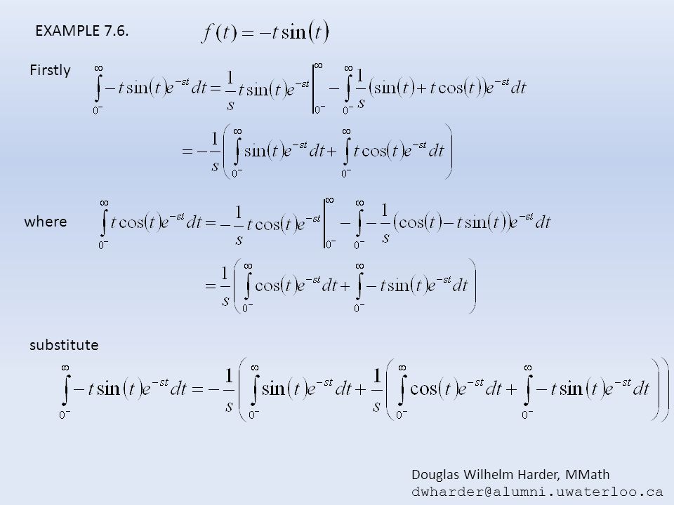
53. EXAMPLE 7.6. Firstly where substitute Douglas Wilhelm Harder, MMath

54. EXAMPLE 7.6.
substitute
therefore

55. THEOREM 7.5 Integration with Respect to s
If there is a real number s0 such that
exists for s>s0, and exists, then
for s>s0, or, equivalently,
EXAMPLE 7.7. To evaluate

56. THEOREM 7.6 Large s Behavior of F(s)
Let f(t) be piecewise continuous on for each finite and of exponential order as , then
(i)
(ii)
Proof : Since f(t) is of exponential order as
then there exist real constants K and c, with K  0 such that
| f(t) |  Kect for all t  T.
Since f(t) is piecewise continuous on
There must be a finite constant M such that | f(t) |  M, on
For all s>c:

57. THEOREM 7.7 Initial-Value Theorem
Let f be continuous and f’ be piecewise continuous on for each finite , and let f and f’ be of exponential order as
then
NOTE:
The utility of this theorem lies in not having to take the inverse of F(s)
in order to find out the initial condition in the time domain. This is
particularly useful in circuits and systems.
Proof : with the stated assumptions on f and f’, it follows that
Since f’ satisfies the conditions of THEOREM 4.7, it follows that
thus

58. EXAMPLE 7.8.
Given
Find f(0)

59. THEOREM 7.8 Final Value Theorem
Let f be continuous and f’ be piecewise continuous on
, and let f and f’ be of exponential order as
then
*Additional Section
NOTE:
It can be used to find the steady-state value of a closed loop system (providing that a steady-state value exists.
Again, the utility of this theorem lies in not having to take the inverse
of F(s) in order to find out the final value of f(t) in the time domain.
This is particularly useful in circuits and systems.
EXAMPLE 7.9.
Suppose
then

60. EXAMPLE 7.10.
Given: .

61. THEOREM 7.9 Transform of Periodic Function
If f is periodic with period T on and piecewise continuous one period, then
EXAMPLE 7.11.
(a)cos(t) is repeated with period 2p (b)cos(t) is repeated with period p
From Douglas Wilhelm Harder,
University of Waterloo.

62. Consider f(t) below: (a) (b)
EXAMPLE 7.12.
Consider f(t) below: (a) (b)
From Douglas Wilhelm Harder,
University of Waterloo.

63. THEOREM 7.10 Scaling in Time
If exists for s>s0, then for any real constant a>0,
for s>s0
*Additional Section
Proof :
EXAMPLE 7.13.

64. THEOREM 7.11 Time delay
Time delays occur due to fluid flow, time required to do an analysis (e.g., gas chromatograph). The delayed signal can be represented as
then
*Additional Section
EXAMPLE 7.14.

65. Common Transform Properties Table
f(t)
F(s)

66. EXAMPLE 7.15
Solve the ODE,
First, take L of both sides of the equation,
Rearrange,
Take L-1,
From Table,

67. References
Schiff. Joel L. The Laplace transform: theory and applications.
Murray. R. SPIEGEL. Schaum’s Outline of Theory and Problems of Advanced Mathematics for Engineers and Scientists.
K.A. Stroud. Engineering Mathematics.
Douglas Wilhelm Harder, Math. University of Waterloo