1. Nonequilibrium Green’s Function Method in Thermal Transport
Wang Jian-Sheng

2. Lecture 1: NEGF basics – a brief history, definition of Green’s functions, properties, interpretation.
Lecture 2: Calculation machinery – equation of motion method, Feynman diagramatics, Dyson equations, Landauer/Caroli formula.
Lecture 3: Applications – transmission, transient problem, thermal expansion, phonon life-time, full counting statistics, reduced density matrices and connection to quantum master equation.

3. References
J.-S. Wang, J. Wang, and J. T. Lü, “Quantum thermal transport in nanostructures,” Eur. Phys. J. B 62, 381 (2008).
J.-S. Wang, B. K. Agarwalla, H. Li, and J. Thingna, “Nonequilibrium Green’s function method for quantum thermal transport,” Front. Phys. (2013).
See also
See also

4. History, definitions, properties of NEGF
Lecture One
History, definitions, properties of NEGF

5. A Brief History of NEGF Schwinger 1961 Kadanoff and Baym 1962
Keldysh 1965
Caroli, Combescot, Nozieres, and Saint-James 1971
Meir and Wingreen 1992

6. Equilibrium Green’s functions using a harmonic oscillator as an example
Single mode harmonic oscillator is a very important example to illustrate the concept of Green’s functions as any phononic system (vibrational degrees of freedom in a collection of atoms) at ballistic (linear) level can be thought of as a collection of independent oscillators in eigenmodes. Equilibrium means that system is distributed according to the Gibbs canonical distribution.

7. Harmonic Oscillator m k
du/dt = sqrt(hbar/(2Omega)) ( - a + a\dagger) (i Omega)

8. Eigenstates, Quantum Mech/Stat Mech

9. Heisenberg Operator/Equation
O: Schrödinger operator
O(t): Heisenberg operator

10. Defining >, <, t, Green’s Functions

11. T, Ť are called super-operator, as it act on the operator, not in the vector of Hilbert space.

12. Retarded and Advanced Green’s functions

13. Fourier Transform
We use the convention that planewave is exp(ik.r – i wt).

14. Plemelj formula, Kubo-Martin-Schwinger condition
P for Cauchy principle value
Valid only in thermal equilibrium

15. Matsubara Green’s Function

16. Nonequilibrium Green’s Functions
By “nonequilibrium”, we mean, either the Hamiltonian is explicitly time-dependent after t0, or the initial density matrix ρ is not a canonical distribution.
We’ll show how to build nonequilibrium Green’s function from the equilibrium ones through product initial state or through the Dyson equation.

17. Definitions of General Green’s functions
Other types such as Matsubara Green’s function or canonical (Kubo) correlation are also used. i = sqrt(-1). The average < … > can be equilibrium or with respect to arbitrary density matrix. For classical systems, G< = G>. 17

18. Relations among Green’s functions
The relation implies two (three?) linearly independent ones, and one independent one only if nonlinear dependence is considered. 18

19. Steady state, Fourier transform
The inverse Fourier transform has a factor of 2 . We use square brackets [ ] to denote Fourier transformed function. 19

20. Equilibrium Green’s Function, Lehmann Representation
Lehmann representation is to expand everything in the eigenstates.

21. Kramers-Kronig Relation
G^a is when z -> w – I eta.

22. Eigen-mode Decomposition
Only for finite system, in equilibrium? See a nice summaryin appendix of Phys Rev B (2009).

23. Pictures in Quantum Mechanics
Schrödinger picture: O, (t) =U(t,t0)(t0)
Heisenberg picture: O(t) = U(t0,t)OU(t,t0) , ρ0, where the evolution operator U satisfies
< . > = Tr(ρ . ). T here denotes time order, assuming t > t’. Anti-time order if t < t’.
See, e.g., Fetter & Walecka, “Quantum Theory of Many-Particle Systems.” 23

24. Calculating correlation
t0 is the synchronization time where the Schrödinger picture and Heisenberg picture are the same. B A t0 t’ t 24

25. Evolution Operator on Contour

26. Contour-ordered Green’s function
Contour order: the operators earlier on the contour are to the right. See, e.g., H. Haug & A.-P. Jauho. τ’ τ t0 26

27. Relation to other Green’s function
σ = + for the upper branch, and – for the returning lower branch. τ’ τ t0 27

28. An Interpretation
This is originally due to Schwinger.
G is defined with respect to Hamiltonian H and density matrix ρ and assuming Wick’s theorem.

29. Calculus on the contour
Integration on (Keldysh) contour
Differentiation on contour
dτ is σdt for integration, but just dt in differentiation. σ is either just the sign + or -, or +1, -1. 29

30. Theta function and delta function
Delta function on contour
where θ(t) and δ(t) are the ordinary theta and Dirac delta functions 30

31. Transformation/Keldysh Rotation
Also properly known as Larkin-Ovchinikov transform, JETP 41, 960 (1975).

32. Convolution, Langreth Rule
The last two equations are known as Keldysh equations.

33. Equation of motion method, Feynman diagrams, etc
Lecture two
Equation of motion method, Feynman diagrams, etc

34. Equation of Motion Method
The advantage of equation of motion method is that we don’t need to know or pay attention to the distribution (density operator) ρ. The equations can be derived quickly.
The disadvantage is that we have a hard time justified the initial/boundary condition in solving the equations.

35. Heisenberg Equation on Contour
The integral on the exponential is from a point tau_1 specified on the contour to tau_2 at a later point on the contour. The integral is along the contour.

36. Express contour order using theta function
Operator A(τ) is the same as A(t) as far as commutation relation or effect on wavefunction is concerned
u uT is a square matrix, and [u, vT] is a matrix formed by (j,k) element [uj, vk]. 36

37. Equation of motion for contour ordered Green’s function
We use the equation of motion d2u/dt2 = -Ku. 37

38. Equations for Green’s functions38

39. Solution for Green’s functions
Note that if ax = b, x = b/a, but not if a = 0, in that case, x = infinity, thus, the Dirac delta function.
c and d can be fixed by initial/boundary condition. 39

40. Feynman diagrammatic method
The Wick theorem
Cluster decomposition theorem, factor theorem
Dyson equation
Vertex function
Vacuum diagrams and Green’s function

41. Handling interaction Transform to interaction picture, H = H0 + Hn
For the concept of pictures and relations among them, see A. L. Fetter and J. D. Walecka, “Quantum theory of many-body systems”, McGraw-Hill, The meaning of t0 and t’ is quite different. t0 is such that three pictures are equivalent, t’ is an arbitrary time. Note that ρ behaves like |><|. 41

42. Scattering operator S
A(t) and B(t’) are in interaction picture (i.e. AI(t) etc). 42

43. Contour-ordered Green’s function
Another possible representation of the result is using Feynman path integral formulation. τ’ τ t0 43

44. Perturbative expansion of contour ordered Green’s function
Every operator is in interaction picture, dropped superscript I for simplicity. The Wick theorem is valid if the expectation < … > is with respect to a quadratic weight. For a proof, see Rammer. 44

45. General expansion rule
Single line
3-line vertex
n-double line vertex
See our review article or Rammer’s book.

46. Diagrammatic representation of the expansion=
+ 2iħ
+ 2iħ
+ 2iħ = +
Due to the last term, G should be read as connected part G_c only in the Dyson equation. 46

47. Self -energy expansion
The self-energy diagrams are obtained by including all doubly or more connected diagrams removing the two external legs from the Green’s function diagrams. For a more systematic exposition of the Feynman-diagrammatic expansion, see Fetter and Welecka. hbar was set to 1 in the diagrams. 47

48. Explicit expression for self-energy
See also figure 3 in J.-S. Wang, X. Ni, and J.-W. Jiang, Phys. Rev. B 80, (2009). 48

49. Junction system, adiabatic switch-on
gα for isolated systems when leads and centre are decoupled
G0 for ballistic system
G for full nonlinear system
HL+HC+HR +V +Hn
HL+HC+HR +V G
Two adiabatic switch-on’s.
HL+HC+HR G0 g
t = − 
Equilibrium at Tα
t = 0
Nonequilibrium steady state established 49 49

50. Sudden Switch-on g t = −  t = ∞ t =t0 50 HL+HC+HR +V +Hn
Green’s function G
Two adiabatic switch-on’s.
HL+HC+HR g
t = − 
Equilibrium at Tα
t = ∞
t =t0
Nonequilibrium steady state established 50 50

51. Three regions 51 51

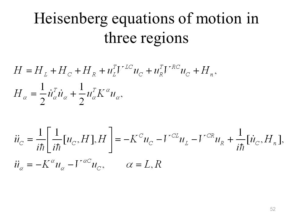
52. Heisenberg equations of motion in three regions52 52

53. Force Constant Matrix

54. Relation between g and G0
Equation of motion for GLC
In obtaining GLC, an arbitrary function satisfying (d/dtau^2 + KL) f = 0 is omitted. Absence of this term is consistent with adiabatic switch-on from Feynman diagrammatic expansion. 54

55. Dyson equation for GCC
In this derivation, we assume Hn = 0. 55

56. Equation of Motion Way (ballistic system)

57. “Partition Function”

58. Diagrammatic Way
Feynman diagrams for the nonequilibrium transport problem with quartic nonlinearity. (a) Building blocks of the diagrams. The solid line is for gC, wavy line for gL, and dash line for gR; (b) first few diagrams for ln Z; (c) Green’s function G0CC; (d) Full Green’s function GCC; and (e) re-sumed ln Z where the ballistic result is ln Z0 = (1/2) Tr ln (1 –gCΣ). The number in front of the diagrams represents extra combinatorial factor.

59. The Langreth theorem
Need to use the relation between G++, G- -, G+-, and G+- with Gr and G<. See Haug & Jauho, page 66. 59

60. Dyson equations and solution
In deriving the last line, we use the fact (gr)-1 g< = 0. 60

61. Energy current
IL is energy flowing out of the left lead into the center. This expression can be proving to be real, no need to take Re. Above equation works for general nonlinear case. 61

62. Landauer/Caroli formula
The symmetrization appears necessary to get the Caroli formula. Caroli formula is valid only for ballistic case where Hn = 0. 62

63. 1D calculation
In the following we give a complete calculation for a simple 1D chain (the baths and the center are identical) with on-site coupling and nearest neighbor couplings. This example shows the general steps needed for more general junction systems, such as the need to calculate the “surface” Green’s functions.

64. Ballistic transport in a 1D chain
Force constants
Equation of motion
The matrix K is infinite in both directions. 64

65. Solution of g
KR is semi-finite, V is nonzero only at the corner. 65

66. Lead self energy and transmission1 ω
ΣR is nonzero only for the lower right corner. 66

67. Heat current and conductance
The last formula σ is called universal conductance. 67

68. General recursive algorithm for g
The algorithm is due to Lopez Sancho et al (1985). Typically, 10 to 20 iterations should be already converged. 68

69. Lecture Three
Applications

70. Carbon nanotube (6,0), force field from Gaussian
Dispersion relation
Transmission
The force constants were symmetrized using the method of Mingo et al (2008). Calculation was performed by Lü Jingtao.
Calculation was performed by J.-T. Lü. 70

71. Carbon nanotube, nonlinear effect
The transmissions in a one-unit-cell carbon nanotube junction of (8,0) at 300K. From J-S Wang, J Wang, N Zeng, Phys. Rev. B 74, (2006).
The nonlinear result may be not correct at the low frequency end. 71

72. u4 Nonlinear model
One degree of freedom (a) and two degrees freedom (b) (1/4) Σ Tijkl ui uj uk ul nonlinear model. Symbols from quantum master equation, lines from self-consistent NEGF. For parameters used, see Fig.4 caption in J.-S. Wang, et al, Front. Phys. Calculated by Juzar Thingna. 1 5 10

73. Molecular dynamics with quantum bath
For more detail, see Phys. Rev. B 80, (2009). Any idea how to generalize this so that quantum mechanics is reproduced exactly?
See J.-S. Wang, et al, Phys. Rev. Lett. 99, (2007);
Phys. Rev. B 80, (2009). 73

74. Average displacement, thermal expansion
One-point Green’s function
The idea of calculating the thermal expansion coefficient this way due to Jiang Jinwu. 74

75. Thermal expansion Left edge is fixed.
Displacement <u> as a function of position x.
as a function of temperature T. Brenner potential is used. From J.-W. Jiang, J.-S. Wang, and B. Li, Phys. Rev. B 80, (2009).
Left edge is fixed. 75

76. Graphene Thermal expansion coefficient
The coefficient of thermal expansion v.s. temperature for graphene sheet with periodic boundary condition in y direction and fixed boundary condition at the x=0 edge.  is onsite strength. From J.-W. Jiang, J.-S. Wang, and B. Li, Phys. Rev. B 80, (2009). 76

77. Phonon Life-Time
For calculations based on this, see, Y. Xu, J.-S. Wang, W. Duan, B.-L. Gu, and B. Li, Phys. Rev. B 78, (2008).
Xu Yong’s formula may have a factor 2 wrong.

78. Transient problems
The IL is valid for 1D chain with spring constant k. Eduardo will present a talk on this topic Friday morning. 78

79. Dyson equation on contour from 0 to t
Contour C
In steady state we use Keldysh contour which is from - to +. But here for transient study, the contour is a finite segment. 79

80. Transient thermal current
The time-dependent current when the missing spring is suddenly connected. (a) current flow out of left lead, (b) out of right lead. Dots are what predicted from Landauer formula. T=300K, k =0.625 eV/(Å2u) with a small onsite k0=0.1k. From E. C. Cuansing and J.-S. Wang, Phys. Rev. B 81, (2010). See also arXiv: 80 80

81. Finite lead problem
Top ↥: no onsite (k0=0), (a) NL = NR = 100, (b) NL=NR=50, temperature T=10, 100, 300 K (black, red, blue). TL=1.1T, TR = 0.9T.
Right ↦: with onsite k0=0.1k and similarly for other parameters. From E. C. Cuansing, H. Li, and J.-S. Wang, Phys. Rev. E 86, (2012). 81 81

82. Full counting statistics (FCS)
What is the amount of energy (heat) Q transferred in a given time t ?
This is not a fixed number but given by a probability distribution P(Q)
Generating function
All moments of Q can be computed from the derivatives of Z.
The objective of full counting statistics is to compute Z(ξ). 82 82

83. A brief history on full counting statistics
L. S. Levitov and G. B. Lesovik proposed the concept for electrons in 1993; rederived for noninteracting electron problems by I. Klich, K. Schönhammer, and others
K. Saito and A. Dhar obtained the first result for phonon transport in 2007
J.-S. Wang, B. K. Agarwalla, and H. Li, PRB 2011; B. K. Agarwalla, B. Li, and J.-S. Wang, PRE 2012. 83

84. Definition of generating function based on two-time measurement
Consistent history quantum mechanics (R. Griffiths). 84

85. Product initial state 85

86. For electron number measurement, the effect to phase a phase, see B. K
For electron number measurement, the effect to phase a phase, see B. K. Agarwalla, B. Li, and J.-S. Wang, “Full-counting statistics of heat transport in harmonic junctions: transient, steady states, and fluctuation theorems,” Phys. Rev. E 85, (2012). 86

87. Schrödinger/Heisenberg/interaction pictures
Schrödinger picture
Heisenberg picture
Interaction picture 87

88. Compute Z in interaction picture
-ξ/2
+ξ/2 88

89. Important result 89

90. Long-time result, Levitov-Lesovik formula90

91. Arbitrary time, transient result91

92. Numerical results, 1D chain
1D chain with a single site as the center.
k= 1eV/(uÅ2), k0=0.1k,
TL=310K, TC=300K, TR=290K. Red line right lead; black, left lead. B. K. Agarwalla, B. Li, and J.-S. Wang, PRE 85, , 2012. 92

93. Cumulants in Finite System
Plot of the culumants of heat <<Qn>> for n=1,2,3, and 4 for one-atom center connected with two finite lead (one-dimensional chain) as a function of measurement time tM. The black and red line correspond to NL =NR =20 and 30, respectively. The initial temperatures of the left, center, right parts are 310K, 360K, and 290K, respective. We choose k=1 eV/(uÅ2) and k0=0.1 eV/(uÅ2) for all particles. From J.-S. Wang, et al, Front. Phys

94. FCS for coupled leads
From H. Li, B. K. Agarwalla, and J.-S. Wang, Phys. Rev. E 86, (2012); H. Li, B. K. Agarwalla, and J.-S. Wang, Phys. Rev. B 86, (2012). For multiple leads, see B. K. Agarwalla, et al, arXiv: 94

95. FCS in nonlinear systems
Can we do nonlinear?
Yes we can. Formal expression generalizes Meir-Wingreen
Interaction picture defined on contour
Some example calculations 95

96. Vacuum diagrams, Dyson equation, interaction picture transformation on contour96

97. Nonlinear system self-consistent results
Single-site (1/4)λu4 model cumulants.
k=1 eV/(uÅ2), k0=0.1k, Kc=1.1k, V LC-1,0=V CR0,1=-0.25k, TL=660 K, TR=410K.
From H. Li, B. K. Agarwalla, B. Li, and J.-S. Wang, arxiv:: 97

98. Quantum Master Equations
When we tried to calculation the reduced density matrix from Dyson expansion, we found that the 2nd order (of the system-bath coupling) diagonal terms do not agree with master equation results, and there are also divergences in higher orders. Similarly, the currents also diverge at higher order. We were quite puzzled. The following is our effort to solve this puzzle and found an expression of the high order current which is finite.

99. Quantum Master Equations
Some detail is in the last section of J.-S. Wang, B. K. Agarwalla, H. Li, and J. Thingna, “Nonequilibrium Green's function method for quantum thermal transport,” Front. Phys. (2013). rho_0 is in fact rho_0^I, i.e., interaction picture one.

100. Unique one-to-one map ρ ↔ ρ0

101. Group & Acknowledgements
Group members: front (left to right) Mr. Zhou Hangbo, Prof. Wang Jian-Sheng, Dr./Ms Lan Jinghua, Mr. Wong Songhan; Back: Mr. Li Huanan, Dr. Zhang Lifa, Dr. Bijay Kumar Agarwalla, Mr. Kwong Chang Jian, Dr. Thingna Juzar Yahya. Picture taking 17 April Others not in the picture: Qiu Hongfei. Thanks also go to Jian Wang, Jingtao Lü, Jin-Wu Jiang, Edardo Cuansing, Meng Lee Leek, Ni Xiaoxi, Baowen Li, Peter Hänggi, Pawel Keblinski.