1. Support Vector Machines

2. RBF-networks
Support Vector Machines
Good Decision Boundary
Optimization Problem
Soft margin Hyperplane
Non-linear Decision Boundary
Kernel-Trick
Approximation Accurancy
Overtraining

5. Gaussian response function
Each hidden layer unit computes
x = an input vector
u = weight vector of hidden layer neuron i

6. Location of centers u The location of the receptive field is critical
Apply clustering to the training set
each determined cluster center would correspond to a center u of a receptive field of a hidden neuron

7. Determining  Following heuristic will perform well in practice
For each hidden layer neuron, find the RMS distance between ui and the center of its N nearest neighbors cj
Assign this value to i

8. The output neuron produces the linear weighted sum
The weights have to be adopted
(LMS)

9. Why does a RBF network work?
The hidden layer applies a nonlinear transformation from the input space to the hidden space
In the hidden space a linear discrimination can be performed
f( )
f( )
f( )
f( )
f( )
f( )
f( )
f( )
f( )
f( )
f( )
f( )
f( )
f( )
f( )
f( )

10. Support Vector Machines
Linear machine
Constructs a hyperplane as the decision surface in such a way that the margin of separation between positive and negative examples is maximized
Good generalization performance
Support vector learning algorithm may construct following three learning machines
Polynominal learning machines
Radial-Basis functions networks
Two-layer perceptrons

11. Two Class Problem: Linear Separable Case
Many decision boundaries can separate these two classes
Which one should we choose?
Class 2
Perceptron learning rule can be used to find any decision boundary between class 1 and class 2
Class 1

12. Example of Bad Decision Boundaries
Class 2
Class 2
Class 1
Class 1

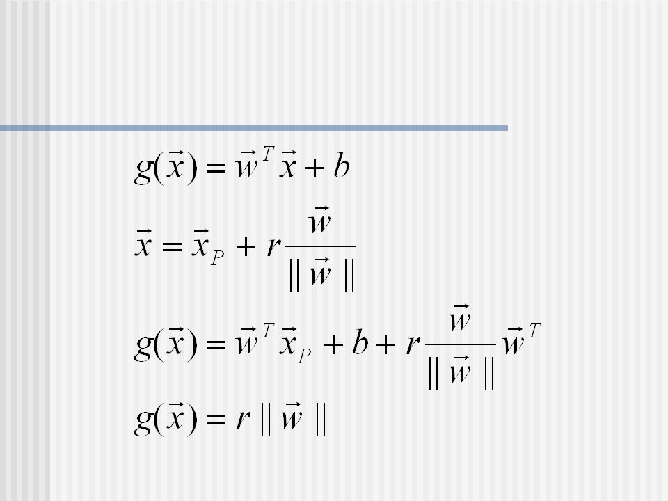
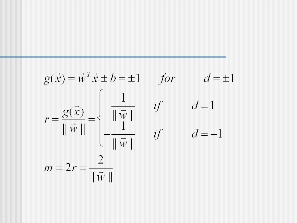
13. Good Decision Boundary: Margin Should Be Large
The decision boundary should be as far away from the data of both classes as possible
We should maximize the margin, m
w/||w|| * (x1-x2) = 2/||w||
Class 2 m
Class 1

16. The Optimization Problem
Let {x1, ..., xn} be our data set and let
yi  {1,-1} be the class label of xi
The decision boundary should classify all points correctly 
A constrained optimization problem

17. The Optimization Problem
Introduce Lagrange multipliers ,
Lagrange function:
Minimized with respect to w and b

18. The Optimization Problem
We can transform the problem to its dual
This is a quadratic programming (QP) problem
Global maximum of ai can always be found
w can be recovered by
Let x(1) and x(-1) be two S.V.
Then b = -1/2( w^T x(1) + w^T x(-1) )

19. A Geometrical Interpretation
Class 2
a8=0.6
a7=0
a2=0
a5=0
a1=0.8
a4=0
So, if change internal points, no effect on the decision boundary
a6=1.4
a9=0
a3=0
Class 1

20. How About Not Linearly Separable
We allow “error” xi in classification
Class 2
Class 1

21. Soft Margin Hyperplane
Define xi=0 if there is no error for xi
xi are just “slack variables” in optimization theory
We want to minimize
C : tradeoff parameter between error and margin
The optimization problem becomes

22. The Optimization Problem
The dual of the problem is
w is also recovered as
The only difference with the linear separable case is that there is an upper bound C on ai
Once again, a QP solver can be used to find ai
Note also, everything is done by inner-products

23. Extension to Non-linear Decision Boundary
Key idea: transform xi to a higher dimensional space to “make life easier”
Input space: the space xi are in
Feature space: the space of f(xi) after transformation
Why transform?
Linear operation in the feature space is equivalent to non-linear operation in input space
The classification task can be “easier” with a proper transformation. Example: XOR
XOR: x_1, x_2, and we want to transform to x_1^2, x_2^2, x_1 x_2
It can also be viewed as feature extraction from the feature vector x, but now we extract more feature than the number of features in x.

24. Extension to Non-linear Decision Boundary
Possible problem of the transformation
High computation burden and hard to get a good estimate
SVM solves these two issues simultaneously
Kernel tricks for efficient computation
Minimize ||w||2 can lead to a “good” classifier
f( )
f( )
f( )
f( )
f( )
f(.)
f( )
f( )
f( )
f( )
f( )
f( )
f( )
f( )
f( )
f( )
f( )
f( )
f( )
Feature space
Input space

25. Example Transformation
Define the kernel function K (x,y) as
Consider the following transformation
The inner product can be computed by K without going through the map f(.)

26. Kernel Trick
The relationship between the kernel function K and the mapping f(.) is
This is known as the kernel trick
In practice, we specify K, thereby specifying f(.) indirectly, instead of choosing f(.)
Intuitively, K (x,y) represents our desired notion of similarity between data x and y and this is from our prior knowledge
K (x,y) needs to satisfy a technical condition (Mercer condition) in order for f(.) to exist

27. Examples of Kernel Functions
Polynomial kernel with degree d
Radial basis function kernel with width s
Closely related to radial basis function neural networks
Sigmoid with parameter k and q
It does not satisfy the Mercer condition on all k and q
Research on different kernel functions in different applications is very active
Despite violating Mercer condition, the sigmoid kernel function can still work

29. Multi-class Classification
SVM is basically a two-class classifier
One can change the QP formulation to allow multi-class classification
More commonly, the data set is divided into two parts “intelligently” in different ways and a separate SVM is trained for each way of division
Multi-class classification is done by combining the output of all the SVM classifiers
Majority rule
Error correcting code
Directed acyclic graph

30. Conclusion SVM is a useful alternative to neural networks
Two key concepts of SVM: maximize the margin and the kernel trick
Many active research is taking place on areas related to SVM
Many SVM implementations are available on the web for you to try on your data set!

31. Measuring Approximation Accuracy
Comparing its output with correct values
Mean squared Error F(w) of the network
D={(x1,t1),(x2,t2), . .,(xd,td),..,(xm,tm)}

33. RBF-networks
Support Vector Machines
Good Decision Boundary
Optimization Problem
Soft margin Hyperplane
Non-linear Decision Boundary
Kernel-Trick
Approximation Accurancy
Overtraining

35. Bibliography
Simon Haykin, Neural Networks, Secend edition Prentice Hall, 1999