1. Persistent Homology and Sensor Networks Persistent homology motivated by an application to sensor nets

2. Outline A word about sensor nets Basic coverage criterion Better coverage criterion using persistence Introduce Persistent Homology Correspondence Theorem Computing the groups! Other Applications

3. A Word About Sensor Nets

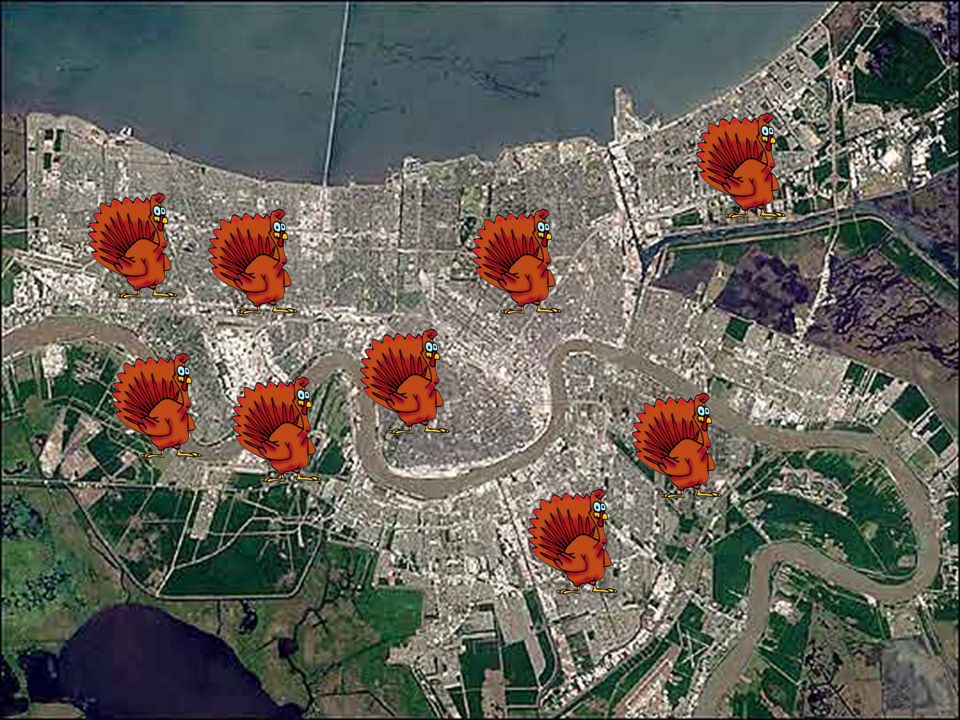
5. August 29, 2005 Hurricane Katrina hits New Orleans

6. Power and Communications Knocked Out

7. Broken Levees

8. City Flooded

9. Inaccessible from the ground

10. Law Enforcement

11. Rescue Workers

19. Replace live turkey with a parachute

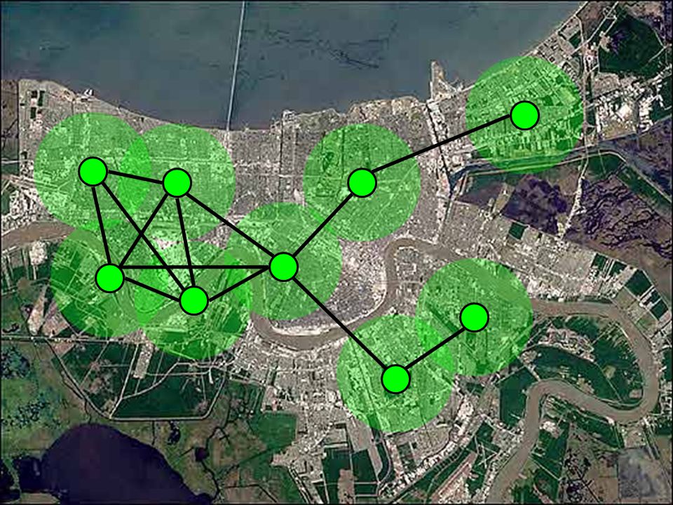
20. Result: Useful sensor network Measure conditions on the ground at many locations Relay messages to and from rescue workers Instant infrastructure Low power/auto-power Cheap!?

21. Other uses of sensor networks Environmental monitoring Security systems Battlefield monitoring and communications Large mechanical systems Find Sarah Connor

23. Hole in sensor coverage area Sarah Connor escapes!

24. Identifying holes in the network De Silva and Ghrist have developed a method for identifying gaps in sensor coverage Method is based on Algebraic Topology Computing and examining Simplical Homology groups Theoretical underpinings allow you to do so much more

25. Basic Coverage Criterion Part 1.2

26. rcrc rbrb The problem to be solved: Each node has sensors that can cover a circular region of radius r c Each node can detect other nodes Within its broadcast radius r b r c ≥ r b /√(3)

27. The problem to be solved: Each node has sensors that can cover a circular region of radius r c Each node can detect other nodes Within its broadcast radius r b r c ≥ r b /√(3) Nodes lie in compact connected planar domain with piecewise linear boundary. Fence nodes at the vertices All fence nodes know their neighbors’ identities and are no more than r b apart

28. What we don’t have: Nodes don’t know their absolute or relative positions All we get is the connectivity graph

29. It would be nice to have the Cech Complex Def: For a collection of sets U ={U  }, the Cech Complex C ( U ) is the simplical complex where each non-empty intersection of (k+1) of the U  correspond to a k-simplex. 3-simplex

30. We have just enough to build the Rips Complex Let X be a collection of points in a metric space Rips complex R  (X) contains a simplex for every collection of points that are pairwise within distance   Even though our domain is planar, a dense graph can lead to simplices with arbitrary dimension In our case, we are building R rb ( X ) Every complete k-subgraph of the communication graph becomes a simplex in the Rips Complex Also, it’s the maximal simplicial complex that has the connectivity graph as its 1-skeleton

31. Picture of a Rips Complex

32. Recap: X  = { set of nodes } r c = sensor radius r b = broadcast radius D = domain to be covered ∂ D = boundary of D X f  = { fence nodes that lie on  D } R  = Rips complex of the communication graph U  = Region covered by the sensors F  = Fence subcomplex  R

33. Theorem (De Silva & Ghrist): For a set of nodes X in a planar domain D satisfying the assumptions (r c, r b, fence nodes etc), the sensor cover U c contains D if there exists [  ]  H 2 ( R, F ) such that ∂  ≠ 0

34. What about a generator of H 2 ( R, F )? A generator will look like some linear combination of 2-simplices i.e. Some triangulation of the domain D

35. Theorem (De Silva & Ghrist): For a set of nodes X in a planar domain D satisfying the assumptions (r c, r b, fence nodes etc), the sensor cover U c contains D if there exists [  ]  H 2 ( R, F ) such that ∂  ≠ 0 But why require ∂  ≠ 0 ?? Why not “if and only if” ??

36. Pitfalls of the Rips complex Bound was r c ≥ r b /√(3) 1/√ (3) ≈ 0.57 Therefore it’s possible to have a rectangle that is completely covered, but not triangulated in the communication graph rbrb rbrb So the conditions of the theorem are sufficient, but not necessary, to guarantee coverage.

37. Pitfalls of the Rips complex It’s possible to have an arrangement of nodes whose Rips complex is the surface of an octahedron. This has non-zero H 2, but its boundary is zero!

38. Better coverage criterion using persistence Part 1.3

39. Eliminating the fence subcomplex The assumption of the nice fence sub-complex is unrealistic Can we replace it with some other assumptions?

40. The new situation: Each node has sensors that can cover a circular region of radius r c Each node can detect its neighbors via a strong signal (r s ) or a weak signal (r w ). r c ≥ r s /√(2) r w ≥ r s √(10) rcrc rsrs rwrw Remember: strong “short” weak “ w long”

41. The new situation (cont…): r c ≥ r s /√(2) r w ≥ r s √(10) Nodes lie in a compact connected domain D in R d Nodes can detect the presence of ∂D within distance r f The restricted domain D-C is connected, where C = {x  D  ||x- ∂D || ≤ r f + r s /√(2) The fence-detection hypersurface  = {x  D  ||x- ∂D || = r f } Has internal injectivity radius ≥ r s /√(2) external injectivity radius ≥ r s

42. The new situation (cont…): rfrf The fence “collar”, C  restricted domain D - C The boundary ∂D Domain D

43. New complexes We get two communication graphs now, corresponding to r s and r w One gives us the “strong” Rips Complex, R s The other gives the “weak” Rips complex R w Note that R s  R w

44. (more) New complexes We also get a subcomplex based on the nodes that lie within r f of ∂D Build this as a subcomplex of R s Call it the (strong) fence subcomplex F s rfrf

45. What we’d like to see Conjecture: For a set of nodes X in a domain D  R d satisfying the new assumptions (r c, r s, r w, r f, fence subcomplex etc), the sensor cover U contains D - C if there exists [  ]  H d ( R s, F s ) such that ∂  ≠ 0

46. Why it fails rfrf By comparing to the “weak” Rips complex, we can see which of these cycles are phantom and which are legitimate It’s possible to get “phantom” d-cycles in the relative homology that have non-zero boundary

47. Theorem (De Silva & Ghrist): For a set of nodes X in a domain D in R d satisfying the new assumptions (r c, r s, r w, r f, fence subcomplex etc), the sensor cover U contains D - C if the homomorphism i * : H d ( R s, F s ) ----> H d ( R w, F w ) induced by the inclusion i: ( R s, F s ) ----> ( R w, F w ) is nonzero.

48. The “Squeezing” Theorem For a set of points X in a domain D  R d R  ( X )  C  ( X )  R  ( X ) whenever  /  ≥ √(2d/(d+1)) Note that for d=2 this means  ≥ 1.15  This means that if you can enlarge (or shrink) the radius of your Rips complex a little, and the complex doesn’t change, then you actually have a Cech complex

49. Persistence Part 2

50. The Usual Homology Have a single topological space, X, and a PID, R Get a chain complex For k=0, 1, 2, … compute H k (X) H k =Z k /B k C k (X)C 1 (X)C 0 (X)C k-1 (X)0 ∂ ∂∂∂∂∂

51. How about a filtration of spaces? X 1  X 2  X 3  …  X n a b a b cd a b cd a b cd a b cd a b cd a, bc, d, ab, bccd, adacabcacd t=0t=1t=2t=3t=4t=5 We restrict to simplical complexes (so we can compute)

52. Leads to a Persistence Complex X 1  X 2  X 3  …  X n C0kC0k C01C01 C00C00 C 0 k-1 0 ∂ ∂∂∂∂∂ C1kC1k C11C11 C10C10 C 1 k-1 0 ∂ ∂∂∂∂∂ CnkCnk Cn1Cn1 Cn0Cn0 C n k-1 0 ∂ ∂∂∂∂∂ Columns are inclusion maps Inclusion is a chain map, and so induces a map on homology

53. Induces a map on homology a b a b cd a b cd a b cd a b cd a b cd a, bc, d, ab, bccd, adacabcacd t=0t=1t=2t=3t=4t=5 For each dimension k=0,1,2,… Consider a generator [  ]  H i k We may want to consider where in the filtration that generator first appears (created), and when it first becomes bounding (destroyed) H0kH0k H1kH1k i*i* H2kH2k i*i* HnkHnk i*i*

54. Concept: P -interval a b a b cd a b cd a b cd a b cd a b cd a, bc, d, ab, bccd, adacabcacd t=0t=1t=2t=3t=4t=5 A P -interval is an ordered pair (i, j) with 0≤i<j ≤∞ Consider a generator [  ]  H i k We can encode information about the creation and destruction time of [  ] as a P -interval For example [ab+bc-ac]  H 1 has P -interval (3, 4)

55. Definition: Persistent Homology a b a b cd a b cd a b cd a b cd a b cd a, bc, d, ab, bccd, adacabcacd t=0t=1t=2t=3t=4t=5 H k i,p = Start with the k-cycles at t=i ZkiZki “fast-forward” the boundaries to some future time, i+p B k i+p Intersect the denominator with Z k i so it’s well-defined  Zki Zki

56. Too much work? a b a b cd a b cd a b cd a b cd a b cd a, bc, d, ab, bccd, adacabcacd t=0t=1t=2t=3t=4t=5 This is interesting, but for an N-step filtration of dimension D, this means we have to compute O(N 2  D) homology groups! And how can we tell what a generator at one time step becomes at the next timestep? We need compatible bases for the whole filtration! H k i,p = ZkiZki B k i+p  Zki Zki

57. Definition: Persistence Module Let R be a commutative PID A persistence module is a collection of R-modules, M i, together with R-module homomorphisms  i such that  i :M i ---> M i+1 M = {M i,  i } A persistence module M is said to be of finite type if the individual M i are finitely generated, and  N such that n ≥ N   i :M i  M i+1

58. Correspondence Theorem Let R be a commutative PID, and M = {M i,  i } a persistence module of finite type over R Define a functor  Where the R-module structure on the M i is the sum of the individual components, and the action of t is given by t·(m 0, m 1, m 2, …) = (0,  0 (m 0 ),  1 (m 1 ),  2 (m 2 ), …) R-persistence modules of finite type Finitely generated non- negatively graded R[t] modules  i=0 ∞  ( M ) =  M i Proof: “the Artin-Rees theory in commutative algebra”?

59. Correspondence Theorem Let R be a commutative PID, and M = {M i,  i } a persistence module over R Define a functor  If R=F is a field, then F[t] is a graded PID and we have a structure theorem for its finitely- generated graded modules R-persistence modules of finite type Finitely generated non- negatively graded R[t] modules  i=0 ∞  ( M ) =  M i i=1 n  =    _i F[t]     _j F[t]/(t n_j ) m j=1 free parttorsion part

60. Example: Homology of a filtration The homology groups H k l (for a fixed k) of a finite filtration {X l }, along with the maps induced by inclusions are a persistence module of finite type. H k = {H k l, i * l } In the corresponding graded R[t] module M=  ( H k ), each stage in the filtration corresponds to a particular degree. a b a b cd a b cd a b cd a b cd a b cd a, bc, d, ab, bccd, adacabcacd t0t0 t1t1 t2t2 t3t3 t4t4 t5t5 The element [ab+bc-ac]  H 1 3 has degree 3 But t·[ab+bc-ac]  0 in H 1 4

61. Visualization: “Barcodes” a b a b cd a b cd a b cd a b cd a b cd a, bc, d, ab, bccd, adacabcacd t0t0 t1t1 t2t2 t3t3 t4t4 t5t5

62. Computing simplicial homology The boundary operators of the chain complex are linear operators operating on chain groups which are free R-modules Therefore they can be represented as matrices relative to some bases. C k (X)C 1 (X)C 0 (X)C k-1 (X)0 ∂ ∂∂∂∂∂ By the standard basis we mean the basis where individual simplices are represented as the unit vectors in R k a b cd C 0 = = 10001000 01000100 00100010 00010001 C 1 = = 1000010000 0100001000 0010000100 0001000010 0000100001

63. Computing simplicial homology 2 The boundary map  k :C k ---> C k-1 is represented by the R-matrix M k a b cd C 0 = = 10001000 01000100 00100010 00010001 C 1 = = 1000010000 0100001000 0010000100 0001000010 0000100001 -1 0 0 -1 -1 1 -1 0 0 0 0 1 -1 0 1 0 0 1 1 0 M 1 =

64. Computing simplicial homology 3 Then M k can be reduced by elementary operations to a matrix, M k in Smith Normal Form a b cd -1 0 0 -1 -1 1 -1 0 0 0 0 1 -1 0 1 0 0 1 1 0 M 1 = ~ abcdabcd ab bc cd ad ac  1 0 0 0... 0 0 0 0  r 0 0 M k = ~ b 1... b r b r+1... b m a 1... a r z 1.... z n-r The  i ’s that are >1 are the torsion coefficients of H k-1 z 1,..., z r are a basis for kerM k = Z k  1 b 1,...,  r b r are a basis for imM k = B k-1 So between M k and M k+1 we have enough information to compute H k, betti numbers 1 0 0 0 0 0 1 0 0 0 0 0 1 0 0 0 0 0 0 0 M 1 = ~ a a+b b+c c+d -ab -bc -cd z1 z2 z1 = ab+bc-ac z2 = ac+cd-ad

65. Computing persistent homology To compute persistent homology over a field, F, do the same thing except work over the ring F[t] a b a b cd a b cd a b cd a b cd a b cd a, bc, d, ab, bccd, adacabcacd t0t0 t1t1 t2t2 t3t3 t4t4 t5t5 Each simplex is assigned a degree according to when it got added to the complex For example, deg(a)=0 deg(abc)=4 The boundary operator can’t map across the grading So for a simplex   C k deg(  ) = deg(∂ k  ) For example, ∂ k  ac) = t 2 ·c - t 3 ·a

66. Computing persistent homology 2 a b a b cd a b cd a b cd a b cd a b cd a, bc, d, ab, bccd, adacabcacd t0t0 t1t1 t2t2 t3t3 t4t4 t5t5 For a given dimension, k, there is a single boundary operator, ∂ k  encoding information for the entire filtration. Note that basis elements are homogenous. -t 0 0 -t 2 -t 3 t -t 0 0 0 0 1 -t 0 t 2 0 0 t t 0 M 1 = abcdabcd ab bc cd ad ac t 0 0 0 0 -t 1 0 0 0 0 -t t 0 0 0 0 -t 0 0 M 1 = ~ dcbadcba cd bc ab z1 z2 z1 = ad - cd - t·bc - t·ab z2 = ac - t 2 ·bc - t 2 ·ab

67. Computing persistent homology 3 a b a b cd a b cd a b cd a b cd a b cd a, bc, d, ab, bccd, adacabcacd t0t0 t1t1 t2t2 t3t3 t4t4 t5t5 t 0 0 0 0 -t 1 0 0 0 0 -t t 0 0 0 0 -t 0 0 M 1 = ~ dcbadcba cd bc ab z1 z2 z1 = ad - cd - t·bc - t·ab z2 = ac - t 2 ·bc - t 2 ·ab Torsion terms in persistent homology! A torsion coefficient t i corresponding to a basis element of degree j gives a term in the persistent homology group:  j F[t]/(t i ) Or in other words, a P -interval (j, i+j) An extra basis element of degree j at the bottom gives a free term:  j F[t] IOW a P -interval (j,∞)

68. Applications When your only tool is persistent homology, every problems starts to look like a filtered simplicial complex 1.That sensor nets thing 2.Point cloud data 3.Dimension estimation