Download presentation
Presentation is loading. Please wait.

1
Warping and Morphing

2
Warping There are two ways to warp an image. The first, called forward mapping, scans through the source image pixel by pixel, and copies them to the appropriate place in the destination image. The second, reverse mapping, goes through the destination image pixel by pixel, and samples the correct pixel from the source image. The most important feature of inverse mapping is that every pixel in the destination image gets set to something appropriate. In the forward mapping case, some pixels in the destination might not get painted, and would have to be interpolated. We calculate the image deformation as a reverse mapping. The problem can be stated "Which pixel coordinate in the source image do we sample for each pixel in the destination image?"

5
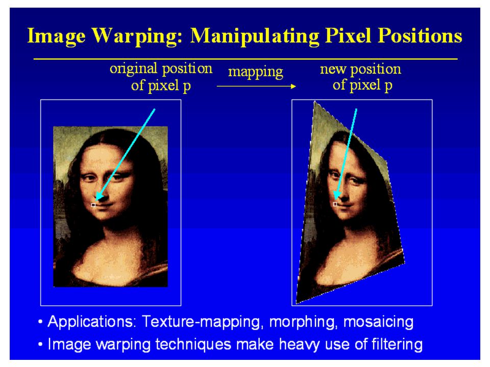
Image Warping Move pixels of image Mapping Resampling
![]()
6
Mapping Define transformation
Describe the destination (x, y) for every location (u, v) in the source image(or vice-versa, if invertible)
 for every location (u, v) in the source image(or vice-versa, if invertible)")
7
Example Mappings Scale by factor x = factor * u y = factor * v

8
Example Mappings Rotate by degrees x = ucos - vsin
y = usin + vcos

9
Other Mappings Any function of u and v x = fx(u, v) y = fy(u, v)
 y = fy(u, v)")
10
Forward Mapping Traverse input pixels Miss/overlap output pixels W
![]()
11
Forward Mapping Iterate over source image
Some destination pixels may not be covered Many source pixels can map to the same destination pixel

12
Inverse Mapping Traverse output pixels Does not waste work W-1
![]()
13
Reverse Mapping Iterate over destination image Must resample source
May oversample, but much simpler!

14
Resampling Evaluate source image at arbitrary (u, v)
(u, v) does not usually have integer coordinates Some kinds of resampling Point resampling Triangle filter Gaussian filter Source Image Destination Image
 does not usually have integer coordinates. Some kinds of resampling. Point resampling. Triangle filter. Gaussian filter. Source Image. Destination Image.")
15
Point Sampling Take value at closest pixel Simple, but causes aliasing
int iu = trunc(u + 0.5); int iv = trunc(v + 0.5); dst(x, y) = src(iu, iv); Simple, but causes aliasing
![]()
16
Triangle Filter Convolve with triangle filter

17
Triangle Filter Bilinearly interpolate four closest pixels
a = linear interpolation of src(u1, v2) and src(u2, v2) b = linear interpolation of src(u1, v1) and src(u2, v1) dst(x, y) = linear interpolation of ‘a’ and ‘b’
![]()
18
Gaussian Filter Convolve with Gaussian filter
Width of Gaussian kernel affects bluriness

19
Filtering Method Comparison
Trade-offs Aliasing versus blurring Computation speed

20
Image Warping Implementation
Reverse mapping for (int x = 0; x < xmax; x++) { for (int y = 0; y < ymax; y++) { float u = fx-1(x, y); float v = fy-1(x, y); dst(x, y) = resample_src(u, v, w); } Source Image Destination Image
 { for (int y = 0; y < ymax; y++) { float u = fx-1(x, y); float v = fy-1(x, y); dst(x, y) = resample_src(u, v, w); } Source Image. Destination Image.")
21
Polynomial Transformation
Geometric correction requires a spatial transformation to invert an unknown distortion function. The mapping functions, U and V , have been universally chosen to be global bivariate polynomial transformations of the form: (20) where aij and bij are constant polynomial coefficients A first degree ( N=1) bivariate polynomial defines those mapping functions that are exactly given by a general 3 x 3 affine transformation matrix .
 where aij and bij are constant polynomial coefficients. A first degree ( N=1) bivariate polynomial defines those mapping functions that are exactly given by a general 3 x 3 affine transformation matrix .")
22
Polynomial Warping In the remote sensing, the polynomial coefficients are not given directly. Instead spatial information is supplied by means of control points, corresponding positions in the input and output images whose coordinates can be defined precisely. In these cases, the central task of the spatial transformation stage is to infer the coefficients of the polynomial that models the unknown distortion. Once these coefficients are known, Eq.20 is fully specified and it is used to map the observed (x,y) points onto the reference ( u,v) coordinate system. This is also called polynomial warping. It is practical to use polynomials up to the fifth order for the transformation function.
 points onto the reference ( u,v) coordinate system. This is also called polynomial warping. It is practical to use polynomials up to the fifth order for the transformation function.")
24
Least – Squares with Ordinary Polynomials
From Equation (20) with N=2, coefficients aij can be determined by minimizing This is achieved by determining the partial derivatives of E with respect to coefficients aij, and equating them to zero. For each coefficient aij, we have : By considering the partial derivative of E with respect to all six coefficients, we obtain the system of linear equations.
 with N=2, coefficients aij can be determined by minimizing. This is achieved by determining the partial derivatives of E with respect to coefficients aij, and equating them to zero. For each coefficient aij, we have : By considering the partial derivative of E with respect to all six coefficients, we obtain the system of linear equations.")
25
Weighted Least Squares
As you see the least-squares formulation is global error measure - distance between control points ( xk, yk) and approximation points ( x,y). The least –squares method may be localized by introducing a weighting function Wk that represents the contribution of control point (xk,yk) on point (x,y) where determines the influence of distant control points and approximating points
 and approximation points ( x,y). The least –squares method may be localized by introducing a weighting function Wk that represents the contribution of control point (xk,yk) on point (x,y) where determines the influence of distant control points and approximating points.")
26
Pseudoinverse Solution
Let a correspondence be established between M points in the observed and reference images. The spatial transformation that approximates this correspondence is chosen to be a polynomial of degree N. In two variables ( x and y) , such a polynomial has K coefficients where For example, a second-degree approximation requires only six coefficients to be solved. In this case , N=2 and K=6. In matrix form: U=WA ; V=WB WTU = WTWA A = (WTW)-1WTU ; B =(WTW)-1WTV
 , such a polynomial has K coefficients where. For example, a second-degree approximation requires only six coefficients to be solved. In this case , N=2 and K=6. In matrix form: U=WA ; V=WB. WTU = WTWA A = (WTW)-1WTU ; B =(WTW)-1WTV.")
27
Warping Summary Reverse mapping is simpler to implement
Different filters trade-off speed and aliasing/blurring Fun and creative warps are easy to implement

28
Image Morphing Animate transition between two images

29
Cross-Dissoving Blend images blend(i, j) = (1-t)src(i, j) + tdst(i, j)
 = (1-t)src(i, j) + tdst(i, j)")
30
Image Morphing Combines warping and cross-dissolving

31
Image Morphing Warping step is the hard one
Aim to align features in images

32
Image Morphing There are two necessary components to morphing algorithms: the user must have a mechanism to establish correspondence between the two images - perhaps as simple as silhouettes from this correspondence, the algorithm must determine a dense pixel correspondence which is the warp algorithm A common technique often used for facial morphing is named feature-based morphing. Important feature are chosen rather than a grid of points that must cover "unimportant" areas. Typical features might be ears, nose, and eyebrows. Lines are drawn in each image and are associated with each other. If there is only one pair of lines, the algorithm produces a purely local change. Therefore, a high spatial density is achieved in areas of interest.

33
Feature-based Morphing
Beier & Neeley use pairs of lines to specify warp Given p in dst image, where is p’ in source image? u is a fraction v is a length(in pixels)
")
34
Feature-based Morphing
The mapping function is simple. An inverse mapping function is used.

35
Feature-based Morphing
If more than one pair of lines is used, the transformations must be blended. Beier and Neeley of Pacific Data Images who developed the technique suggested the use of weight. (NOTE: Beier-92.pdf work).
.")
36
Warping with One Line Pair
What happens to the ‘F’?

37
Warping with Multiple Line Pairs
Use weighted combination of points defined by each pair of corresponding lines p’ is a weighted average

38
Weighting Effect of Each Line Pair
To weight the contribution of each line pair where Length[i] is the length of L[i] dist[i] is the distance from X to L[i] a, b, p are constants that control the warp

39
Warping Pseudocode WarpImage(Image, L’[], L[]) begin
foreach destination pixel p do psum = (0, 0) wsum = (0, 0) foreach line L[i] in destination do p’[i] = p transformed by (L[i], L’[i]) psum = psum + p’[i] * weight[i] wsum += weight[i] end p’ = psum / wsum Result(p) = Image(p’)
![Warping Pseudocode WarpImage(Image, L’[], L[]) begin](http://slideplayer.com/slide/4035209/13/images/39/Warping+Pseudocode+WarpImage%28Image%2C+L%E2%80%99%5B%5D%2C+L%5B%5D%29+begin.jpg "foreach destination pixel p do. psum = (0, 0) wsum = (0, 0) foreach line L[i] in destination do. p’[i] = p transformed by (L[i], L’[i]) psum = psum + p’[i] * weight[i] wsum += weight[i] end. p’ = psum / wsum. Result(p) = Image(p’)")
40
Morphing Pseudocode GenerateAnimation(Image0, L0[], Image1, L1[])
begin foreach intermediate frame time t do for i = 1 to number of line pairs do L[i] = line t-th of the way from L0[i] to L1[i] end Warp0 = WarpImage(Image0, L0, L) Warp1 = WarpImage(Image1, L1, L) foreach pixel p in FinalImage do Result(p) = (1-t)Warp0 + tWarp1
![Morphing Pseudocode GenerateAnimation(Image0, L0[], Image1, L1[])](http://slideplayer.com/slide/4035209/13/images/40/Morphing+Pseudocode+GenerateAnimation%28Image0%2C+L0%5B%5D%2C+Image1%2C+L1%5B%5D%29.jpg "begin. foreach intermediate frame time t do. for i = 1 to number of line pairs do. L[i] = line t-th of the way from L0[i] to L1[i] end. Warp0 = WarpImage(Image0, L0, L) Warp1 = WarpImage(Image1, L1, L) foreach pixel p in FinalImage do. Result(p) = (1-t)Warp0 + tWarp1.")
41
Morphing Summary Specifying correspondences Warping Blending

42
Graphical Objects and Metamorphosis
Object O1 Object O2 Metamorphosis Geometric Data Set Geometric Data Set Geometry Alignment Attributes Attributes Attribute Interpolation

43
Warping Pipeline Generation of attributes Deform Adjust
Transformation of geometry Generation of attributes

44
Morphing Pipeline Deform Adjust Blend Adjust Deform

45
Warping Morphing Warping and Morphing Single object
Specification of original and deformed states Morphing Two objects Specification of initial and final states

46
Warping and Morphing http://www-2.cs.cmu.edu/~seitz/vmorph/vmorph.html

Similar presentations


>")


. 2D preobrazba dekle-tiger.>")

 Slides are from RPI Registration Class.>")


 the inverse perspective transformation which is dependent on the focal length.>")


