Download presentation
Presentation is loading. Please wait.

1
AoN Session 2

2
Highlight a number of cells at the top of the page. Then with the cursor over these cells right click. Scroll down to the format cell.

3
Click on the ‘alignment’ tab. Tick the merge cell tab press the ok button

4
Add a meaning full title use the format options to format the text to 16 point Arial

5
Add three column titles; Name, Shoe size and height. Move the cursor up to the boundary between the C & D double click the left button

6
Add the names of the people in your group to the first column

7
Add the shoe size of the group in the next column

8
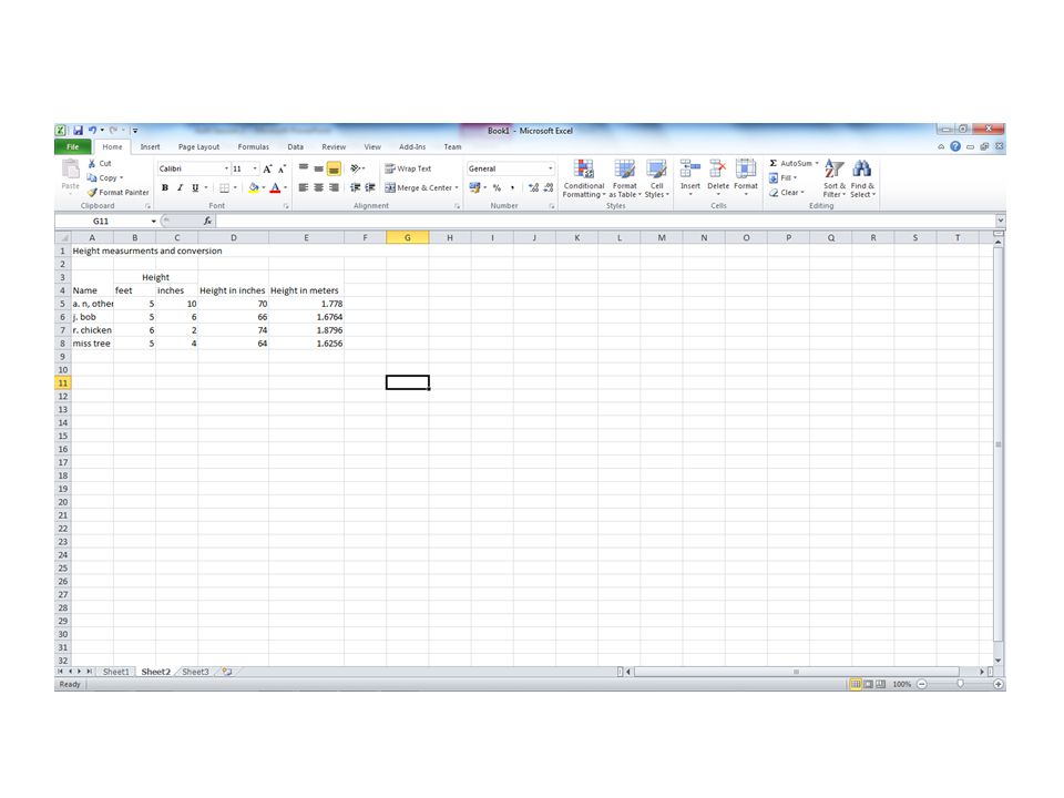
Click on the sheet two tab. Create the table shown here.

9
Add the feet and inches headings under the height heading.

10
Click back to sheet 1. Place the cursor on the cell containing the first name press and hold the left button drag the cursor down to the last name. Place the cursor over the highlighted area and right click once. Click the copy button.

11
Click back to sheet 2. Place the cursor on the cell you want the first name copied to. Right click to bring up the menu bar. Click the paste button.

12
Measure the height of your class mates in feet and inches. Enter the data into your spread sheet.

14
In cell under height in inches enter the following formula All formulas start with ‘=Sum’ this tells the program that there is a calculation that it needs to perform. All information to be calculated need to be with in brackets. The sum in the green brackets will be calculated first. Click on the cell yon want to perform the calculation on then multiply * by 12 (because there are 12 inches to a foot) The sum in the black brackets will be performed second. Once the first calculation has been performed add + the second cell and close the bracket, this tells the program the calculations are complete.
 The sum in the black brackets will be performed second. Once the first calculation has been performed add + the second cell and close the bracket, this tells the program the calculations are complete..")
15
FunctionMathematical symbol Excel symbol Add++ Subtract-- Divide÷/ Multiplyx*

16
Copy the cell

17
Highlight the next cells in the column using the left mouse button. Press the right button once to bring up the menu. Paste the formula using the indicated button on the menu. This pasts the formula into the cells and will calculate the correct amounts for the data in the cells

18
We are going to use the following formula to convert the measurements in inches to meters Start with ‘=sum’ as before open two brackets. Click on the cell you want to perform the conversion on and multiply it by 25.4 (there are 25.4mm in an inch) Now divide the number you have just calculated by 1000 as the number is in mm and you want it in meters. (there are 1000mm in a meter.
 Now divide the number you have just calculated by 1000 as the number is in mm and you want it in meters. (there are 1000mm in a meter..")
19
Enter the formula in to the cell. Once the formula is entered copy and paste the formula into the other cells as before

21
Highlight the cells with the measurements in. Click on the decrease decimal button once, to reduce the number to two decimal places

22
Copy the height measurements from the cells in sheet two, and paste them in to the height cells in sheet one.

23
You are now going to arrange the class by order of height. Highlight the heights of the students.

24
Click on the sort and filter tab. Then press the sort smallest to largest button.

25
A dialogue box will open and offer you two choices click the ‘expand the selection ‘ button then press sort

26
You will see that the heights are now in order and the names have changed correspondingly

27
We are now going to calculate the Mean, Median, Mode and range of your heights. Enter the titles Mean, Mode, Median & Range

28
Highlight and merge four columns and two rows above the mean, mode, median & range. Add title statistical analysis

29
Highlight the column of heights

30
Click the ‘AutoSum’ button. This will add all of the figures up in that column.

31
In the cell next to mean start the formula with =Sum( then click on to the cell with the height total in it this will enter the cell name into the formula. Use the divide symbol “/” and enter the number of people in your data set. Close bracket and press return. Display your mean to two decimal places.

32
In the mode box enter your mode.

33
If the data in your set is odd the mode is the middle number. If the date set is even then you will need to add the two middle numbers together and divide the sum by two.

35
For the range cell start by =sum( then subtract the smallest number in your data set from the largest number in the data set.

36
Repeat the statistical analysis on the shoe size data

37
Highlight the data table and click on the insert tab

38
Click on the column tab in the graph section of the menu Choose the 2-D compare graph.

39
Click on the graph and move the cursor over the corner until it changes to a double arrow, press and hold down the left mouse button and drag the graph until it is larger.

40
Click on the graph, then click on the design tab this will bring up the chart layout ‘ribbon’

41
Click on the ‘add chart title’ tab. Highlight the chart title and type in a meaning full title

42
Click on the ‘layout’ tab then click the ‘Axis Titles’ button

43
Scroll down to the ‘Primary Horizontal Axis Title’ and click on the ‘Title Below Axis’ button

44
Repeat the process for the vertical axis

45
Check that the spread sheet is correctly formatted (capitol letters, punctuation, and general layout) Perform a calculation check on each of the calculation types that you have done.
 Perform a calculation check on each of the calculation types that you have done.")
Similar presentations


. Is a spreadsheet application designed to take advantage of the windows graphical interface MICROSOFT EXCEL.>")


>")
![1 Introduction to Excel Chapter 2. 2 Wrapping Text Steps to wrap text in one cell: Type the amount of text that will fit within a cell [alt] + [enter]](/22/6384148/big_thumb.jpg "1 Introduction to Excel Chapter 2. 2 Wrapping Text Steps to wrap text in one cell: Type the amount of text that will fit within a cell [alt] + [enter]>")

