1. Multifactor Experiments November 26, 2013 Gui Citovsky, Julie Heymann, Jessica Sopp, Jin Lee, Qi Fan, Hyunhwan Lee, Jinzhu Yu, Lenny Horowitz, Shuvro Biswas

2. Outline Two-Factor Experiments with Fixed Crossed Factors 2 k Factorial Experiments Other Selected Types of Two-Factor Experiments

3. Two-Factor Experiments with Fixed Crossed Factors

4. First, single factor Comparison of two or more treatments (groups) Single treatment factor Example: A study to compare the average flight distances for three types of golf balls differing in the shape of dimples on them: circular, fat elliptical, thin elliptical Treatments circular, fat elliptical, thin elliptical Treatment factor type of ball

5. Single factor continued

6. Two-Factor Experiments With Fixed Crossed Factors Two fixed factors, A with a ≥ 2 levels and B with b ≥ 2 levels ab treatment combinations If there are n observations obtained under each treatment combination ( n replicates), then there is a total of abn experimental units

7. Two-Factor Experiments With Fixed Crossed Factors Example: Heat treatment experiment to evaluate the effects of a quenching medium (two levels: oil and water) and quenching temperature (three levels: low, medium, high) on the surface hardness of steel 2 x 3 = 6 treatment combinations If 3 steel samples are treated for each combination, we have N = 18 observations

8. Model and Estimates of its Parameters Let y ijk =k th observation on the (i,j) th treatment combination, i=1,2,…,a, j=1,2,…,b, and k=1,2,…,n. Let random variable Y ijk correspond to observed outcome y ijk. Basic Model: and independent where

9. Table format

10. Parameters Grand Mean: i th Row Average: j th Column Average: ( i,j ) th Row Column Interaction i th Row Main Effect: j th Column Main Effect:

11. Least Squares Estimates

12. Variance Sample variance for ( i, j ) th cell is: Pooled estimate for σ 2 :

13. Example Experiment to study how mechanical bonding strength of capacitors depends on the type of substrate (factor A) and bonding material (factor B). 3 substrates: Al 2 O 3 with bracket, Al 2 O 3 no bracket, BeO no bracket 4 types of bonding material: Epoxy I, Epoxy II, Solder I and Solder II Four capacitors were tested at each factor level combination

14. Example continued Pooled sample variance:

15. Example continued: Sample Means

16. Example continued: Other Model Parameters

17. Two- Way Analysis of Variance We define the following sum of squares:

18. Analysis of Variance Degrees of Freedom: SST: N – 1 SSA: a – 1 SSB: b – 1 SSAB: ( a – 1)( b – 1) SSE: N – ab SST = SSA + SSB + SSAB + SSE. Similarly, the degrees of freedom also follow this identity, i.e.

19. Analysis of Variance

20. Hypothesis Test We test three hypotheses: Not all If all interaction terms are equal to zero, then the effect of one factor on the mean response does not depend on the level of the other factors.

21. When do we reject H 0 ? Use F -statistics to test our hypotheses by taking the ratio of the mean squares to the MSE. Reject We test the interaction hypothesis H 0AB first.

22. Summary (Table 13.5) Source of Variation (Source) Sum of Squares (SS) Degrees of Freedom (d.f.) Mean Square (MS) F Main Effects A a – 1 Main Effects B b – 1 Interaction AB ( a – 1)( b – 1) Error N – ab Total N – 1

23. Example: Bonding Strength of Capacitors Data Capacitors; input Bonding $ Substrate $ Strength @@; Datalines; Epoxy1 Al203 1.51 Epoxy1 Al203 1.96 Epoxy1 Al203 1.83 Epoxy1 Al203 1.98 … ; proc GLM plots=diagnostics data=Capacitors; TITLE "Analysis of Bonding Strength of Capacitors"; CLASS Bonding Substrate; Model Strength = Bonding | Substrate; run;

24. Bonding Strength of Capacitors ANOVA Table At α =0.05, we can reject H 0B and H 0AB but fail to reject H 0A. The main effect of bonding material and the interaction between the bonding material and the substrate are both significant. The main effect of substrate is not significant at our α.

25. Main Effects Plot Definition : A main effects plot is a line plot of the row means of factor and A and the column means of factor B.

26. Interaction Plot

27. Model Diagnostics with Residual Plots Why do we look at residual plots? Is our constant variance assumption true? Is our normality assumption true?

28. 2 k Factorial Experiments

29. 2 k factorial experiments is a class of multifactor experiments consists of design in which each factor is studied at 2 levels. If there are k factors, then we have 2 k treatment combinations 2-factor and 3-factor experiments can be generalized to >3-factor experiments

30. 2 2 experiment 2 2 Experiment: experiment with factors A and B, each at two levels. ab = (A high, B high) a = (A high, B low) b = (A low, B high) (1) = (A low, B low)

31. 2 2 experiment cont’d Y ij ~ N(µ i, σ 2 ) i = (1), a, b, ab j = 1, 2, …, n Assume a balanced design with n observations for each treatment combinations, denote these observations by y ij

32. 2 2 experiment cont’d

33. The least square estimates of the main effects and the interaction effects are obtained by replacing the treatment means by the corresponding cell sample means.

34. Contrast Coefficients for Effects in a 2 2 Experiment Treatment combinati on Effect IABAB (1)+--+ a++-- b+-+- ab++++ *Notice that the term-by-term products of any two contrast vectors equal the third one 2 2 experiment cont’d

35. 2 3 experiment 2 3 Experiment: experiment with factors A, B, and C with n observations. Y ij ~ N(µ i, σ 2 ), i = (1), a, b, ab, c, ac, bc, abc j = 1, 2, …, n.

36. 2 3 experiment cont’d

37. Contrast coefficients for Effects in a 2 3 Experiment Treatment Combination Effect IABABCACBCABC (1)+--+-++- a++----++ b+-+--+-+ ab++++---- c+--++--+ ac++--++-- bc+-+-+-+- abc++++++++ 2 3 experiment cont’d

38. 2 3 experiment example Factors affecting bicycle performance: Seat height (Factor A): 26" (-), 30" (+) Generator (Factor B): Off (-), On(+) Tire Pressure (Factor C): 40 psi (-), 55 psi (+)

39. 2 3 experiment example cont’d Travel times from Bicycle Experiment FactorTime (Secs.) ABCRun 1Run 2Mean ---515452.5 +--414342.0 -+-546057.0 ++-444343.5 --+504849.0 +-+39 39.0 -++535152.0 +++414442.5

40. 2 3 experiment example cont’d significant

41. 2 k experiment 2 k experiments, where k>3. n iid observations y ij ( j = 1,2,… n ) at the i th treatment combination and its sample mean y i ( i = 1,2,…, 2 k ) has the following estimated effect.

42. Statistical Inference for 2 k Experiments Basic Notations and Derivations

43. CI and Hypotheses Test with t Test

44. Hypotheses Test with F Test

45. Sums of Squares for Effects The effects are mutually orthogonal contrasts.

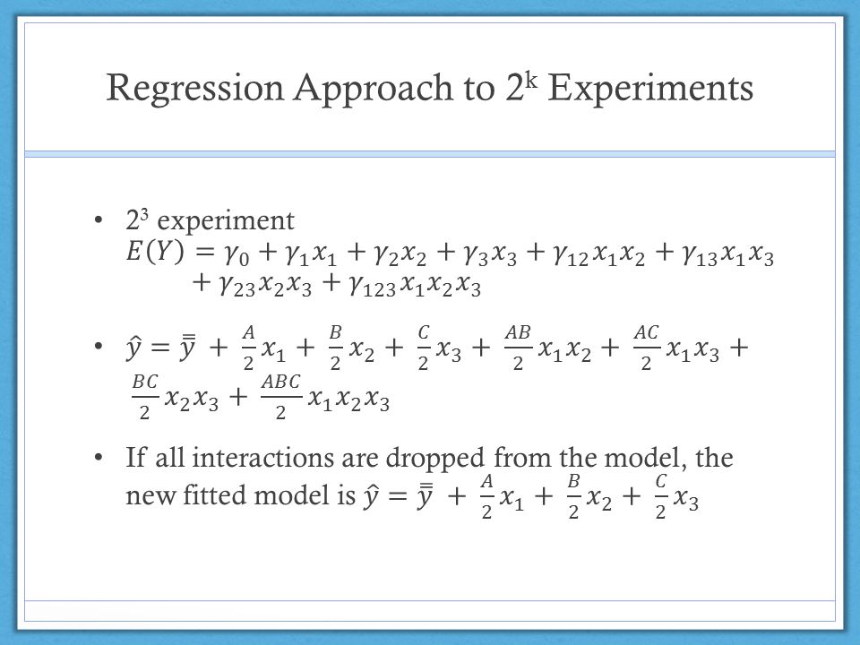
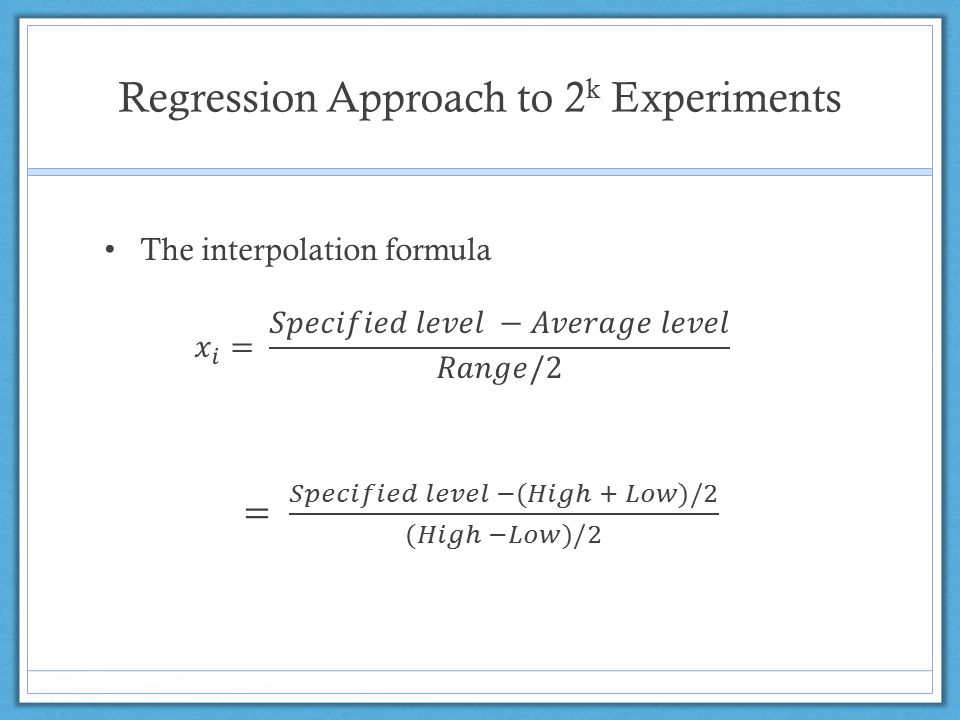
46. Regression Approach to 2 k Experiments

49. Bicycle Example: Main Effects Model

50. Sums of squares for omitted interactions effects

51. Bicycle Example: Residual Diagnostics To check model assumptions proc glm plots=diagnostics data = biker; class A B C; model travel= A|B|C; run; Normality Equal error variance

52. Single Replicated Case Unusual response? Noise? Spoiling the results?

53. Single Replicated Case Effect Sparsity principle If number of effects is large (e.g. k= 4, 15 effects), a majority of them are small ~N (0, σ 2 ), few a large and more influential ~ (u≠0, σ 2 ) Reduced model retaining only significant effects, omitting non-significant ones Obtain sums of squares for omitted effects => pooled error sum of squares (SSE) (Error due to ignoring negligible effects) Error d.f. = # pooled omitted effects MSE = SSE/error d.f. Perform formal statistical inferences

54. Other Types of Two- Factor Experiments Section 13.3

55. Two-Factor Experiments with (Crossed and) Mixed Factors A is fixed factor with a levels B is random factor with b levels Assume a balanced design with n ≥ 2 obs’s at each of (a x b) treatment combinations

56. Example: Compare three testing laboratories Material tested comes in batches Several samples from each batch tested in each laboratory Laboratories represent a fixed factor Batches represent a random factor Two factors are crossed, since samples are tested from each batch in each laboratory Model?

57. Mixed Effects Model Y ijk = µ + τ i + ß j + ( τ ß) ij + Є ijk  µ, τ i are fixed parameters  ß j, ( τ ß) ij are random parameters  Є ijk i.i.d. N(0, σ 2 ) random errors

58. The (Probability) Distribution of the Random Effects

59. Variance Components Model

60. Expected Mean Squares E(MSA) = σ 2 + n σ 2 AB + n Σ i a τ i 2 /(a-1) E(MSB) = σ 2 + n σ 2 AB + an σ 2 B E(MSAB) = σ 2 + n σ 2 AB E(MSE) = σ 2

61. Unbiased estimators of variance components

62. Common tests H 0A : τ 1 = … = τ a = 0 vs. H 1A : At least one τ i ≠ 0 H 0B : σ 2 B = 0 vs. H 1B : σ 2 B > 0 H 0AB : σ 2 AB = 0 vs. H 1AB : σ 2 AB > 0

63. Common tests: results Reject H 0A if F A = MSA/MSAB > f a-1,(a-1)(b-1), α Reject H 0B if F B = MSB/MSAB > f b-1,(a-1)(b-1), α Reject H 0AB if F AB = MSAB/MSE > f (a-1)(b-1),v, α

64. Two-Factor Experiments w. Nested and Mixed Factors Model: Where,

65. Two-Factor Experiments w. Nested and Mixed Factors Orthogonal Decomposition of Sum of Squares

66. Two-Factor Experiments w. Nested and Mixed Factors ANOVA Table

67. Illustrative Example Consider the Following Experiment: ~ A  Concentration of Reactant ~ B  Concentration of Catalyst

68. Analysis with SAS Code

69. Analysis with SAS Selected Output

70. Summary Two factor experiments with multiple levels Model: We can decompose the Sum of Squares as: And compute test statistics under Ho, as:

71. Summary 2^k Factorial Experiments k factors, 2 levels each Calculate the Sum of Squares due to an effect as

72. Acknowledgements Tamhane, Ajit C., and Dorothy D. Dunlop. "Analysis of Multifactor Experiments." Statistics and Data Analysis: From Elementary to Intermediate. Upper Saddle River, NJ: Prentice Hall, 2000. Cody, Ronald P., and Jeffrey K. Smith. "Analysis of Variances: Two Independent Variables." Applied Statistics and the SAS Programming Language. 5th ed. Upper Saddle River, NJ: Prentice Hall, 2006. Prof. Wei Zhu Previous Presentations