1. PREDICTING MLB CAREER SALARIES Stephanie Aube Mike Tarpey Justin Teal

2. OBJECTIVE  To determine the best model for estimating how much a given Major League Baseball player will make in salary throughout his career, based on current batting and fielding statistics.  It’s relatively clear that Major League Baseball and other professional sports pay for performance. The idea is to come up with a way to statistically forecast a career salary, and what variables are best for this task.

3. OBTAINING DATA Primary Source: Lahman Baseball Database Sean Lahman  Compiled every major baseball statistic including salaries for players between 1985-2012  Database won awards from baseball and sporting magazines

4. VARIABLES  PlayerID – Name of player (the ID key)  SumOfSalary – The sum of a player’s salary over their career  Weight  Height  Bats (right, left, switch)  Throws (right, left)  SumOfAB – Career At Bats  SumOfR – Career Runs Scored  SumOfH – Career Hits  SumOf2B, SumOf3B, SumOfHR – Career doubles, triples, and homeruns  SumOfRBI – Career Runs Batted In  SumOfSB – Career Stolen Bases  SumOfSO – Career Strike Outs  SumOfPO – Career Put Outs (defensive)  SumOfA – Career Assists (devensive)  SumOfE – Career Errors (defensive)  SumOfDP – Career Double Plays (defensive)  SumOfCS – Career Times Caught Stealing (baserunning)  Country of Birth  State of Birth (if born in US)  Hall of Fame (binary, 1=admitted)  School (binary, 1=played in college)

5. DATA SUMMARY  4,512 total players considered  56.69% played in college  7.402% eventually voted into HOF  Average player size: 196.8 pounds, just under 6’2”  62.97% of the sample bats right handed

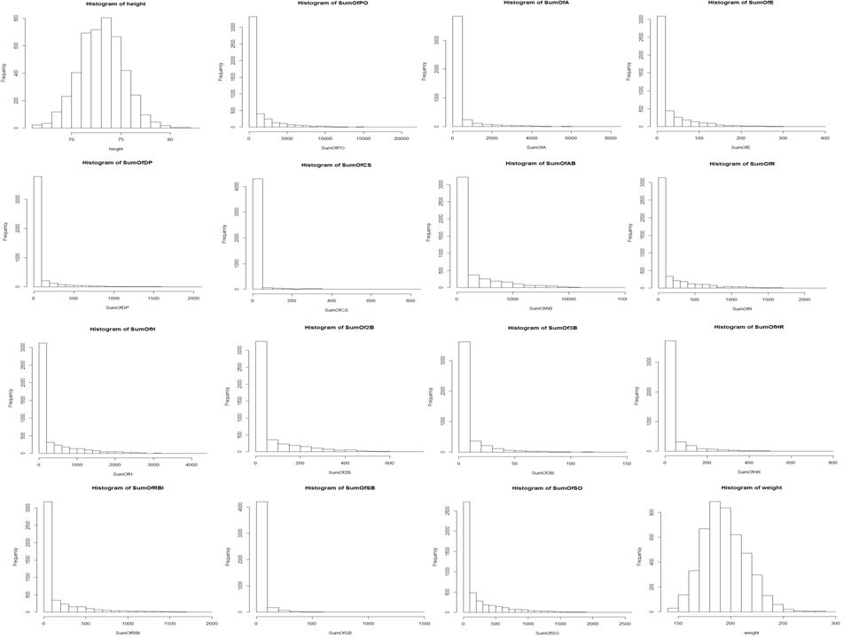
6. DATA STRUCTURE  Our response variable is heavily skewed to the right, so during model selection transformation was considered and eventually implemented

7. EXPLANATORY VARIABLES  Because most explanatory variables are career sum variables, nearly every one is right skewed. This can be attributed to two factors:  Very few major league players start in almost every game for their team; it’s only those that do that rack up large statistics. Some players may only be called up from lower leagues for a few games to substitute in for a hurt superstar.  Specialty players (home run hitters, better fielders)  This will be further considered during model selection.

9. MODEL SELECTION  Full model used as a starting point  Includes every variable with the exception of state and country of birth

10. FULL MODEL

11. FULL MODEL FLAWS  Only about 43% of the response variable, career salary, is explained by the model  Some coefficients are thrown off by heavy collinearity. More AB = less money should not be an expected result of the model  Log transformations on the many right-skewed variables can help model fit  Can advanced statistics help to build a better model?

12. SABRMETRICS  Society of American Baseball Research  Statistics that provide better indication of player output  Now widely used in MLB

13. CREATED VARIABLES  Batting Average on Balls in Play (BABIP)  BABIP = (SumOfH – SumOfHR)/(SumOfAB – SumOfSO – SumOfHR)  Player Runs Percentage Adjusted (PRPA)  PRPA = (SumOfRBI – SumOfSO)/(SumOfAB)  Slugging Percentage (SLUG)  SLUG = (SumOfH + 2*SumOf2B + 3*SumOf3B + 4*SumOfHR)/(SumOfAB)

14. NEW FULL MODEL  Includes all 20 variables from original model plus 3 SABRmetrics  BAPIP significant at.01 level  SLUG significant at.001 level  8/9 offensive variables significant  RBI not significant  4/4 defensive variables significant

15. MODEL NARROWING  StepAIC both from full to reduced and reduced to full selected same model  From 23 variables, removed Bats (left, right, switch), BinaryHOF, PRPA

16. SALARY TRANSFORMATION  SumOfSalary is right skewed  Ran same model on log(SumOfSalary)  4/10 offensive variables significant  4/4 defensive variables significant

17. SABER TRANSFORMATION

18.  Chose log(SLUG + 1) to replace SLUG  Added SLUG 2 to model

19. INTERACTION VARIABLES  Players with multiple skills should be paid more  SLUG and SumOfA  SumOfHR and SumOfSB  Only interaction between SLUG and SumOfA deemed significant

20. DEALING WITH SKEWNESS  All variables were at least slightly skewed  Took natural log of every explanatory variable and SumOfSalary (dependent variable)  Did not transform variables Weight, Height, Throws, HOF, School, BABIP

21. RESIDUALS VS. FITTED FOR NEW BEST MODEL

22. QQ PLOT OF NEW BEST MODEL

23. COLLINEARITY – INITIAL FULL MODEL

24. COLLINEARITY – FULL MODEL PLUS SABER

25. COLLINEARITY – FINAL MODEL

26. INTERESTING FINDINGS  RBIs had no statistical significance  Advanced statistics proved to be significant in player salary analysis, but not team analysis  Weight much more significant than height  Many variables in final model  All defensive statistics are significant, but not all offensive

27. FUTURE INVESTIGATIONS  How do variables other than player statistics influence salary?  Team  Years in League  Year with Team  Age

28. SUMMARY  Career salaries are predictable using various batting and fielding statistics  Many player statistics are vital in predicting salaries – higher valued players are well rounded

29. QUESTIONS?