1. SHORT-TERM SCHEDULING PLANNING, SCHEDULING, AND CONTROLLING INTERMITTENT- FLOW OPERATIONS IN THE MANUFACTURING AND SERVICE SECTORS Applied Management Science for Decision Making, 1e © 2012 Pearson Prentice-Hall, Inc. Philip A. Vaccaro, PhD

2.  Each job or job batch travels through a series of work centers, each of which performs a particular task. Intermittent-Flow Operations SALIENT FEATURES

3.  Work centers are grouped by major processing function. Intermittent-Flow Operations SALIENT FEATURES

4.  Each job or job batch has its own unique route through the system. Intermittent-Flow Operations SALIENT FEATURES

5. Intermittent-Flow Operations SALIENT FEATURES  Job processing times at each work center are estimated based on similar past jobs and worker experience

6. Intermittent-Flow Operations  Work centers are grouped by function.  Each job or job batch has its own unique route through the system.  Job processing times at each work center are estimated based on similar past jobs and worker experience.  Workers are highly skilled and flexible. SALIENT FEATURES

7. A AA An Intermittent-Flow Operation Work Center A Work Center B Work Center E Work Center C Work Center D Work Center F cuttingdrillinginspecting sandingpaintingpackaging JOB ENTERS HERE AS RAW WOOD AND HARDWARE FINISHED JOB LEAVES HERE CARPENTRY SHOP EXAMPLE

8. Evaluating all incoming jobs to see which work centers they must pass through in order to be completed. Short-Term Scheduling THE BIG PICTURE

9. Arranging all jobs scheduled for each work center in a specific processing order chosen to meet the shop’s performance goals. Short-Term Scheduling THE BIG PICTURE

10. Evaluating all incoming jobs to see which work centers they must pass through in order to be completed. Arranging all jobs scheduled for each work cen- ter in a specific processing order chosen to meet shop performance goals. Developing detailed start / finish times for each job at each work center.

11. Short-Term Scheduling History  Developed by Henry Gantt, a school teacher by training and later an engineer.  Refined and expanded on the existing body of production and cost control techniques.  Developed the Gantt Chart in 1914 for scheduling and con- trolling production and major projects. Henry Laurence Gantt 1861 - 1919

12. Gantt Chart Accomplishments  WORLD WAR I NAVAL SHIPS ( 1917 )  HOOVER DAM ( 1931 )  MANHATTAN PROJECT ( 1942 )  INTERSTATE HIGHWAY SYSTEM ( 1956 ) Dr. Robert Oppenheimer and General Kenneth Nichols THE GANTT CHART WAS THE PRECURSOR OF PERT/CPM: TODAY’S POPULAR TECHNIQUE FOR MANAGING MAJOR PROJECTS IN GOVERNMENT AND INDUSTRY

13. Short-Term Scheduling Steps I.Aggregate Planning II.Loading III.Priority Sequencing IV.Detailed Scheduling V.Dispatching

14. Aggregate Planning  Identify a quasi-unit that best reflects the firm’s overall output of goods and services  Multiply the quasi-unit forecast by the quasi- unit resource requirements. BRIEF REVIEW THESE STEPS WILL DETERMINE THE NUMBER AND TYPE OF WORK CENTERS, EQUIPMENT, PERSONNEL, PARTS, AND SUPPLIES THAT THE FIRM MUST INVEST IN

15. Number of Vehicles to be Repaired ( in quasi-units ) Average Consumption of Resources, Human and Non-Human ( per quasi-unit ) Total Resource Requirements Over Life of the Aggregate Plan  Number of Mechanics  Number of Vehicle Lifts  Size of the Parts Department  Number and Types of Equipment AUTOMOBILE DEALERSHIP REPAIR FACILITY EXAMPLE

16. Short-Term Scheduling Steps I.Aggregate Planning II.Loading III.Priority Sequencing IV.Detailed Scheduling V.Dispatching

17. LOADING ALSO KNOWN AS SHOP LOADING or MACHINE LOADING The assignment and commitment of arriving jobs to one or more work centers for the day, week, or month, based on job needs.

18. Gantt Chart for Loading WEEKLY SCHEDULE – DEPARTMENT 3985: MODEL SHOP SCHEDULE 3/16 - 22 WORKCENTERMONTUESWEDTHURFRISAT Machining Fabrication Assembly Testing Packaging D D D D A B B B C C C E E E F F

19. The Gantt Chart for Loading  Shows the specific jobs assigned to each work center for the day, week, or month at a glance.  The color bars show the estimated processing times for each job at each work center.

20. The Gantt Chart for Loading  Does not show the exact start and finish times for each job at each center.  Does not show the exact order in which each job will be processed at each center.

21. Short-Term Scheduling Steps I.Aggregate Planning II.Loading III.Priority Sequencing IV.Detailed Scheduling V.Dispatching

22. PRIORITY SEQUENCING THE ORDER IN WHICH JOBS WAITING AT EACH WORK CENTER WILL BE PROCESSED THE ORDER OF PROCESSING SELECTED WILL BEST MEET MANAGEMENT’S SHOP GOALS

23. Priority Sequence Rules Average job completion time Number of setups Setup costs Work-in-process inventory levels Utilization of equipment Idle time Idle time costs Shop productivity Customer delivery time WILL HAVE AN IMPACT ON THE FOLLOWING ( AND MORE )

24. A Few Priority Sequence Rules OVER 36 TO CHOOSE FROM SPTSPT shortest processing time FIFOFIFO first in - first out LIFOLIFO last in - first out SSSS static slack CRCR critical ratio FISFSFISFS first in system - first served ( ALSO KNOWN AS DD, DUE DATE )

25. Priority Sequence Rules NEW PERFORMANCE CRITERIA 1. Average job completion time 2. Labor or machine utilization 3. Average number of jobs in the system 4. Average number of late days per job We evaluate priority sequence rules using one or more of the following criteria:

26. Possible Job Shop Goals  Internal Shop Efficiency  Customer Service  Mix of Both

27. Internal Shop Efficiency To promote this goal, the firm should evaluate priority sequence rules that: - maximize utilization of labor and equipment - minimize the average number of jobs in the system, that is, the work-in-process inventory

28. Customer Service To promote this goal, the firm should evaluate priority sequence rules that: - minimize average job lateness ( tardiness )

29. Efficiency & Customer Service To promote both of these goals, the firm should evaluate priority sequence rules that: - minimize average job completion time

30.  There are currently about a dozen priority sequence rules that support the goal of internal shop efficiency.  We evaluate those dozen rules using two particular performance criteria only. 1. “MAXIMIZE UTILIZATION of workers and equipment” 2. “MINIMIZE WORK-in-PROCESS INVENTORY”  We select the rule that best satisfies those two criteria. Theconnectionbetween shop goals andprioritysequencerules

31.  There are currently about a dozen priority sequence rules that support the goal of customer service.  We evaluate those dozen rules using one particular performance criterion only: “MINIMIZE JOB LATENESS”  We select the rule that best satisfies that criterion. Theconnectionbetween shop goals andprioritysequencerules

32.  There are currently about a dozen priority sequence rules that support the goal of efficiency and service.  We evaluate those dozen rules using one particular performance criterion only. “ MINIMIZE AVERAGE JOB COMPLETION TIME”  We select the rule that best satisfies that criterion. Theconnectionbetween shop goals andprioritysequencerules

33. Priority Sequence Rule Evaluation TEXT EXAMPLE  Assume that this job shop has only one work center.

34. Priority Sequence Rule Evaluation TEXT EXAMPLE  Assume that this work center can only process one job at a time. job at a time.

35. Priority Sequence Rule Evaluation TEXT EXAMPLE  Assume that processing time can be labor or machine time. or machine time.

36. Priority Sequence Rule Evaluation TEXT EXAMPLE  Assume it is the 1 st day of the month.

37. Priority Sequence Rule Evaluation TEXT EXAMPLE  Assume five ( 5 ) jobs are waiting to be done.

38. Priority Sequence Rule Example THE FIVE JOBS JOBS JOB PROCESS TIMES JOB DEADLINES ( tentative ) A5 Days10 th Day B10 Days15 th Day C2 Days5 th Day D8 Days12 th Day E6 Days8 th Day

39. Shortest Processing Time (SPT) THE JOB PROCESSING ORDER JOB PROCESS ORDER TIMECOMPLETIONTIME JOB DEADLINE ( tentative ) JOBLATENESS C2 Days2 nd Day5 th Day0 Days A5 Days7 th Day10 th Day0 Days E6 Days13 th Day8 th Day5 Days D8 Days21 st Day12 th Day9 Days B10 Days31 st Day15 th Day16 Days 5 Jobs31 Days74 Days-30 Days 1 Completion Time, or Flow Time = Job Waiting Time + Job Processing Time

40. First-In, First Out ( FIFO ) THE JOB PROCESSING ORDER JOB PROCESS ORDER TIMECOMPLETIONTIME JOB DEADLINE ( tentative ) JOBLATENESS A5 Days5th Day10th Day0 Days B10 Days15th Day 0 Days C2 Days17 th Day5 th Day12 Days D8 Days25th Day12 th Day13 Days E6 Days31 st Day8 th Day23 Days 1 5 Jobs31 Days93 Days-48 Days Completion Time, or Flow Time = Job Waiting Time + Job Processing Time

41. First-in-System, First-Served (FSFS) JOBS ARE LINED UP BY DUE DATE JOB PROCESS ORDER TIMECOMPLETIONTIME JOB DEADLINE ( tentative ) JOBLATENESS C2 Days2nd Day5th Day0 Days E6 Days8th Day 0 Days A5 Days13 th Day10 th Day3 Days D8 Days21st Day12 th Day9 Days B10 Days31 st Day15 th Day16 Days 5 Jobs31 Days75 Days-28 Days 1 Completion Time, or Flow Time = Job Waiting Time + Job Processing Time

42. Static Slack Computations JOB DEADLINE DATE – CURRENT DATE – JOB PROCESS TIME JOB A : 10 th day – 1 st day – 5 days = 4 days JOB B : 15 th day – 1 st day – 10 days = 4 days JOB C : 5 th day – 1 st day – 2 days = 2 days JOB D : 12 th day – 1 st day – 8 days = 3 days JOB E : 8 th day – 1 st day – 6 days = 1 day THE JOB WITH THE SMALLEST STATIC SLACK IS DONE FIRST

43. JOB PROCESS ORDER TIMECOMPLETIONTIME JOB DEADLINE ( tentative ) JOBLATENESS E6 Days6th Day8th Day0 Days C2 Days8th Day5th Day3 Days D8 Days16 th Day12 th Day4 Days A5 Days21st Day10 th Day11 Days B10 Days31 st Day15 th Day16 Days 5 Jobs31 Days82 Days-34 Days 1 Static Slack - ( SS ) Completion Time, or Flow Time = Job Waiting Time + Job Processing Time

44. Critical Ratio Computations DEADLINE DATE – CURRENT DATE REMAINING PROCESSING TIME JOB A : ( 10 th – 1 st ) / 5 days = 1.80 JOB B : ( 15 th – 1 st ) / 10 days = 1.40 JOB C : ( 5 th – 1 st ) / 2 days = 2.00 JOB D : ( 12 th – 1 st ) / 8 days = 1.37 JOB E : ( 8 th – 1 st ) / 6 days = 1.16 AS THE CRITICAL RATIO GETS SMALLER, THE JOB GETS A HIGHER PRIORITY

45. JOB PROCESS ORDER JOB PROCESS TIME COMPLETION TIME JOB DEADLINE ( tentative ) JOB LATENESS E6 Days6th Day8th Day0 Days D8 Days14th Day12th Day2 Days B10 Days24 th Day15 th Day9 Days A5 Days29th Day10 th Day19 Days C2 Days31 st Day5 th Day26 Days 5 Jobs31 Days104 Days-56 Days 1 Critical Ratio - CR Completion Time, or Flow Time = Job Waiting Time + Job Processing Time

46. Summary Tabulations Priority Sequence Rule Total Job Processing Time ( in days ) Total Job Completion Time ( in days ) Total Job Lateness ( in days ) SPT317430 FIFO319348 FSFS317528 SS318234 CR3110456

47. Average Job Completion Time Total Flow Time / Number of Jobs SPT Rule 74 days / 5 jobs = 14.8 days FIFO Rule 93 days / 5 jobs = 18.6 days FSFS (DD) 75 days / 5 jobs = 15.0 days STATIC SLACK 82 days / 5 Jobs = 16.4 days CRITICAL RATIO 104 days / 5 Jobs = 20.8 days

48. Labor / Machine Utilization Total Processing Time / Total Flow Time SPT Rule 31 days / 74 days = 42.00% FIFO Rule 31 days / 93 days = 33.3% FSFS (DD) 31 days / 75 days = 41.33% STATIC SLACK 31 days / 82 days = 37.8% CRITICAL RATIO 31 days / 104 days = 29.81%

49. Average Number of Jobs in the System Total Flow Time / Total Processing Time SPT Rule 74 days / 31 days = 2.39 jobs FIFO Rule 93 days / 31 days = 3.0 jobs FSFS (DD) 75 days / 31 days = 2.42 jobs STATIC SLACK 82 days / 31 days = 2.65 jobs CRITICAL RATIO 104 days / 31 days = 3.35 jobs

50. Average Number of Late Days per Job SPT Rule 30 days / 5 jobs = 6.0 days FIFO Rule 48 days / 5 jobs = 9.6 days FSFS ( DD ) 28 days / 5 jobs = 5.6 days STATIC SLACK 34 days / 5 jobs = 6.8 days CRITICAL RATIO 56 days / 5 jobs = 11.2 days Total Late Days / Number of Jobs

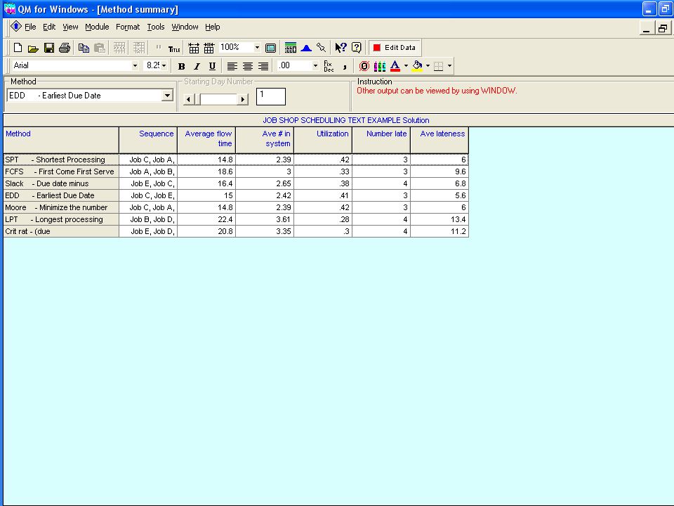
51. Performance Summary RULEAVERAGECOMPLETETIMEUTILIZATION AVER. NO. JOBS IN SYSTEMAVERAGEJOBLATENESSNUMBER OF JOBS LATEMAXIMUMJOBLATENESS SPT 14.8 Days 42.00%2.39 Jobs 6.0 Days3 16 Days FIFO 18.6 Days 33.33%3.00 Jobs 9.6 Days323 Days SS 16.4 Days 37.80%2.65 Jobs 6.8 Days416 Days CR 20.8 Days 29.81%3.35 Jobs 11.2 Days 426 Days DDATE 15.0 Days 41.33%2.42 Jobs 5.6 Days316 Days PRIORITY SEQUENCE RULE EVALUATION

52. Performance Summary RULEAVERAGECOMPLETETIMEUTILIZATION AVER. NO. JOBS IN SYSTEMAVERAGEJOBLATENESSNUMBER OF JOBS LATEMAXIMUMJOBLATENESS SPT 14.8 Days 42.00%2.39 Jobs 6.0 Days3 16 Days FIFO 18.6 Days 33.33%3.00 Jobs 9.6 Days323 Days SS 16.4 Days 37.80%2.65 Jobs 6.8 Days416 Days CR 20.8 Days 29.81%3.35 Jobs 11.2 Days 426 Days DDATE 15.0 Days 41.33%2.42 Jobs 5.6 Days316 Days PRIORITY SEQUENCE RULE EVALUATION

53. Postscript  The SPT rule always minimizes average job completion time ( flow time ) and the average number of. jobs in the system.

54. Postscript   The DDATE rule always minimizes average job lateness and total job lateness.

55. Postscript   FIFO ( FCFS ) does not score well on most criteria but neither does it score poorly. It does however appear fair to customers which is important in service sector systems.

56. Job Shop w / QM for Windows

57. We Scroll To JOB SHOP SCHEDULING

60. There Are Five ( 5 ) Jobs To Be Processed There Is Only One ( 1 ) Machine In Each Work Center Jobs Labeled A,B,C, etc.

61. The Data Input Table Appears

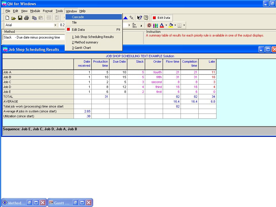
62. We Schedule Under The SPT Priority Sequence Rule. It is the 1 st Day of the Month. Estimated Processing Times Are Entered Under “ Production Time” & Job Deadlines Are Entered Under “Due Date”

63. Under the SPT priority sequence rule, the order of processing is: 1 st Job C, 2 nd Job A, 3 rd Job E, 4 th Job D, 5 th Job B The Performance Criteria

64. SUMMARY STATISTICS for Seven ( 7 ) Priority Sequence Rules

65. Performance Summary RULEAVERAGECOMPLETETIMEUTILIZATION AVER. NO. JOBS IN SYSTEMAVERAGEJOBLATENESSNUMBER OF JOBS LATEMAXIMUMJOBLATENESS SPT 14.8 Days 42.00%2.39 Jobs 6.0 Days3 16 Days FIFO 18.6 Days 33.33%3.00 Jobs 9.6 Days323 Days SS 16.4 Days 37.80%2.65 Jobs 6.8 Days416 Days CR 20.8 Days 29.81%3.35 Jobs 11.2 Days 426 Days DDATE 15.0 Days 41.33%2.42 Jobs 5.6 Days316 Days PRIORITY SEQUENCE RULE EVALUATION

66. The Gantt Loading Chart for One ( 1 ) Work Center

67. First Come, First Serve Priority Sequence Rule Analysis

71. Earliest Due Date Priority Sequence Rule Analysis

74. Static Slack Priority Sequence Rule Analysis

78. Critical Ratio Priority Sequence Rule Analysis

82. Short-Term Scheduling Steps I.Aggregate Planning II.Loading III.Priority Sequencing IV.Detailed Scheduling V.Dispatching

83. Gantt Chart for Detailed Scheduling Conveys all loading gantt chart data Indicates the exact start and finish times for each job at each work center Allows real-time tracking of all jobs at each work center Provides the basis for customer delivery dates Indicates scheduled downtime for repair and maintenance Indicates time blocks reserved for important emergency jobs

84. Gantt Chart for Detailed Scheduling WEEKLY SCHEDULE – DEPARTMENT 3985: MODEL SHOP SCHEDULE 3/16 - 22 WORKCENTERMONTUESWEDTHURFRISAT Machining Fabrication Assembly Testing Packaging D D D D A B B B C C C E E E F F SCHEDULED DOWN TIME FOR MAINTENANCE AND SPECIAL JOBS - SCHEDULED DOWN TIME FOR MAINTENANCE AND SPECIAL JOBS

85. Job Status At-A-Glance W ork CenterMondayTuesdayWednesday MACHINING FABRICATION ASSEMBLY SCHEDULED TIME - JOB “B” SCHEDULED TIME - JOB “M” SCHEDULED TIME - JOB “R”

86. Job Status At-A-Glance W ork CenterMondayTuesdayWednesday MACHINING FABRICATION ASSEMBLY CURSOR DENOTES REAL TIME ACTUAL PROGRESS JOB B JOB M JOB R SCHEDULED TIME JOB B IS BEHIND SCHEDULE AS OF LATE MORNING TUESDAY

87. Job Status At-A-Glance W ork CenterMondayTuesdayWednesday MACHINING FABRICATION ASSEMBLY CURSOR DENOTES REAL TIME ACTUAL PROGRESS JOB B JOB M JOB R SCHEDULED TIME JOB M IS AHEAD OF SCHEDULE AS OF LATE MORNING TUESDAY

88. Job Status At-A-Glance W ork CenterMondayTuesdayWednesday MACHINING FABRICATION ASSEMBLY CURSOR DENOTES REAL TIME ACTUAL PROGRESS JOB B JOB M JOB R SCHEDULED TIME JOB R IS EXACTLY ON SCHEDULE AS OF LATE MORNING TUESDAY

89. Short-Term Scheduling Steps I.Aggregate Planning II.Loading III.Priority Sequencing IV.Detailed Scheduling V.Dispatching

90. Dispatching The formal release of the completed job to the customer by the last work center that processed it. by the last work center that processed it.

91. Short-Term Scheduling Tactics Applied Management Science for Decision Making, 1e © 2012 Pearson Prentice-Hall, Inc. Philip A. Vaccaro, PhD

93. The Assignment Algorithm A loading technique for committing two or more jobs to two or more workers or machines in a single work center. With one job assigned to each processor only ! Applied Management Science for Decision Making, 1e © 2012 Pearson Prentice-Hall, Inc. Philip A. Vaccaro, PhD

94. Characteristics Streamlined version of  Streamlined version of the transportation algorithm the transportation algorithm

95. A Transportation Algorithm Tableau Warehouse 1 Warehouse 2 Warehouse 3 Factory A Factory B Factory C 3 3 $3 $4 $9 $7 $12$15 $17 $8 $5 From To 1 1 1 111Demand Availability ONE UNIT SHIPPED FROM EACH SOURCE - ONE UNIT RECEIVED AT EACH DESTINATION

96. A Transportation Algorithm Solution Warehouse 1 Warehouse 2 Warehouse 3 Factory A Factory B Factory C 3 3 $3 $4 $9 $7 $12$15 $17 $8 $5 From To 1 1 1 111Demand Availability 1 1 1 THE OPTIMAL SOLUTION - TOTAL COST = $20.00

97. An Assignment Algorithm Tableau Warehouse 1 Warehouse 2 Warehouse 3 Factory A Factory B Factory C $3 $4 $9 $7 $12$15 $17 $8 $5 From To THE “DEMAND “ ROW & “AVAILABILITY ” COLUMN ARE ELIMINATED

98. An Assignment Algorithm Tableau Worker 1 Worker 2 Worker 3 Job A Job B Job C $3 $4 $9 $7 $12$15 $17 $8 $5 From To  SHOWS ONLY THE COSTS OF PERFORMING EACH JOB UNDER EACH WORKER  ASSIGNABLE JOBS AND WORKERS CAN REPLACE FACTORIES AND WAREHOUSES

99. An Assignment Algorithm Solution Worker 1 Worker 2 Worker 3 Job A Job B Job C $3 $4 $9 $7 $12$15 $17 $8 $5 From To THE OPTIMAL SOLUTION - TOTAL COSTS ARE 20.00

100. Characteristics  Guarantees an optimal solution since it is a solution since it is a linear programming linear programming model model

101. Characteristics  Also known as the Hungarian Method, Flood’s Technique, and the Reduced Flood’s Technique, and the Reduced Matrix Method Matrix Method NAMED AFTER MERRILL MEEKS FLOOD, FAMED OPERATIONS RESEARCHER INDUSTRIAL ENGINEER Ph.D, Princeton, 1935

102. Characteristics  Determines the most efficient assignment of jobs to workers assignment of jobs to workers and machines or vice-versa and machines or vice-versa

103. Assignment Examples COURSES TERRITORIES TABLES CLIENTS MECHANICS SALESPERSONS WAITSTAFF CONSULTANTS AUTOMOBILES INSTRUCTORS

104. HISTORY “ Eugene Egervary Denes Konig “ Fundamental mathematics developed at the University of Budapest in 1932 The Assignment Algorithm is also called the Hungarian Method in their honor

105. HISTORY Developed in its current form Developed in its current form by Harold Kuhn, PhD by Harold Kuhn, PhD Princeton, at Bryn Mawr Princeton, at Bryn Mawr College in 1955 College in 1955 ( 1925 - )

106. Model Assumptions Employed only when all workers or machines  Employed only when all workers or machines are capable of processing all arriving jobs are capable of processing all arriving jobs

107. Model Assumptions Employed only when all workers or machines  Employed only when all workers or machines are capable of processing all arriving jobs are capable of processing all arriving jobs  Dictates that only 1 job be assigned to each worker / machine, and vice-versa worker / machine, and vice-versa

108. Model Assumptions Employed only when all workers or machines  Employed only when all workers or machines are capable of processing all arriving jobs are capable of processing all arriving jobs  Dictates that only 1 job be assigned to each worker / machine, and vice-versa worker / machine, and vice-versa  Total number of arriving jobs must equal the total number of available workers / machines total number of available workers / machines

109. Possible Performance Criteria Profit maximization Cost minimization Idle time minimization Job completion time minimization

110. The Assignment Matrix Worker 1 Worker 2 Worker 3 Worker 4 Job A $20$25$22$28 Job B $15$18$23$17 Job C $19$17$21$24 Job D $25$23$24 These cells contain the labor costs of a particular worker performing a particular job

111. Assignment Algorithm Steps STEP ONE - ROW REDUCTION SUBTRACT THE SMALLEST NUMBER IN EACH ROW FROM ALL THE OTHER NUMBERS IN THAT ROW

112. The Assignment Matrix Worker 1 Worker 2 Worker 3 Worker 4 Job A $20$25$22$28 Job B $15$18$23$17 Job C $19$17$21$24 Job D $25$23$24 THE SMALLEST NUMBER IN EACH ROW

113. The Assignment Matrix Worker 1 Worker 2 Worker 3 Worker 4 Job A $0$5$2$8 Job B $0$3$8$2 Job C $2$0$4$7 Job D $2$0$1

114. The Assignment Matrix Worker 1 Worker 2 Worker 3 Worker 4 Job A $0$5$2$8 Job B $0$3$8$2 Job C $2$0$4$7 Job D $2$0$1

115. Assignment Algorithm Steps STEP TWO - COLUMN REDUCTION SUBTRACT THE SMALLEST NUMBER IN EACH COLUMN FROM ALL THE OTHER NUMBERS IN THAT COLUMN

116. The Assignment Matrix Worker 1 Worker 2 Worker 3 Worker 4 Job A $0$5$2$8 Job B $0$3$8$2 Job C $2$0$4$7 Job D $2$0$1 THE SMALLEST NUMBER IN EACH COLUMN

117. The Assignment Matrix Worker 1 Worker 2 Worker 3 Worker 4 Job A $0$5$1$7 Job B $0$3$7$1 Job C $2$0$3$6 Job D $2$0 THE SMALLEST NUMBER IN EACH COLUMN

118. The Assignment Matrix Worker 1 Worker 2 Worker 3 Worker 4 Job A $0$5$1$7 Job B $0$3$7$1 Job C $2$0$3$6 Job D $2$0 ROW AND COLUMN REDUCTION PRODUCE THE REDUCED MATRIX IT IS ALSO CALLED AN OPPORTUNITY COST MATRIX

119. Assignment Algorithm Steps STEP THREE - ATTEMPT ALL ASSIGNMENTS ATTEMPT TO MAKE ALL THE REQUIRED MINIMUM COST ASSIGNMENTS ONLY THOSE CELLS CONTAINING “ 0 ” OPPORTUNITY COSTS ARE CANDIDATES FOR MINIMUM COST ASSIGNMENTS

120. The Assignment Matrix Worker 1 Worker 2 Worker 3 Worker 4 Job A 0517 Job B 0371 Job C 2036 Job D 2000 THE OPPORTUNITY COST MATRIX WE CAN NOW DROP THE DOLLAR SIGNS

121. The Assignment Matrix Worker 1 Worker 2 Worker 3 Worker 4 Job A 0517 Job B 0371 Job C 2036 Job D 2000 ATTEMPT TO MAKE FOUR MINIMUM COST ASSIGNMENTS NON-PERMITTED ASSIGNMENT - X X XX

122. The Assignment Matrix Worker 1 Worker 2 Worker 3 Worker 4 Job A 0517 Job B 0371 Job C 2036 Job D 2000 JOB “ B “ WAS NOT ABLE TO BE ASSIGNED NON-PERMITTED ASSIGNMENT - X X XX

123. Assignment Algorithm Steps STEP FOUR - EMPLOY THE “H”-FACTOR TECHNIQUE IF ALL REQUIRED ASSIGNMENTS CANNOT BE MADE, USE THE “H” - FACTOR TECHNIQUE IT CREATES MORE “ 0 “ CELLS, WHICH IN TURN, INCREASES THE CHANCES OF MAKING ALL THE REQUIRED ASSIGNMENTS

124. The Assignment Matrix Worker 1 Worker 2 Worker 3 Worker 4 Job A 0517 Job B 0371 Job C 2036 Job D 2000 COVER ALL ZEROS WITH THE MINIMUM NUMBER OF LINES - VERTICAL and / or HORIZONTAL WE CAN COVER THREE ( 3 ) ZEROS WITH A LINE ACROSS ROW “ D “

125. The Assignment Matrix Worker 1 Worker 2 Worker 3 Worker 4 Job A 0517 Job B 0371 Job C 2036 Job D 2000 COVER ALL ZEROS WITH THE MINIMUM NUMBER OF LINES - VERTICAL and / or HORIZONTAL WE CAN COVER TWO MORE ZEROS WITH A LINE DOWN COLUMN “ 1 “

126. The Assignment Matrix Worker 1 Worker 2 Worker 3 Worker 4 Job A 0517 Job B 0371 Job C 2036 Job D 2000 COVER ALL ZEROS WITH THE MINIMUM NUMBER OF LINES - VERTICAL and / or HORIZONTAL WE CAN COVER THE REMAINING ZERO WITH A LINE DOWN COLUMN “ 2 “

127. The Assignment Matrix Worker 1 Worker 2 Worker 3 Worker 4 Job A 0517 Job B 0371 Job C 2036 Job D 2000 COVER ALL ZEROS WITH THE MINIMUM NUMBER OF LINES - VERTICAL and / or HORIZONTAL WE CAN ALTERNATELY COVER THE LAST ZERO WITH A LINE ACROSS ROW “ C “

128. The Assignment Matrix Worker 1 Worker 2 Worker 3 Worker 4 Job A 0517 Job B 0371 Job C 2036 Job D 2000 THE “ H “ FACTOR IS THE LOWEST UNCOVERED NUMBER THE “ H “ FACTOR EQUALS “ 1 “ IN THIS PARTICULAR PROBLEM

129. The Assignment Matrix Worker 1 Worker 2 Worker 3 Worker 4 Job A 0517 Job B 0371 Job C 2036 Job D 2000 ADD THE “ H “ FACTOR TO THE CRISS-CROSSED NUMBERS

130. The Assignment Matrix Worker 1 Worker 2 Worker 3 Worker 4 Job A 0517 Job B 0371 Job C 3036 Job D 3000 ADD THE “ H “ FACTOR TO THE CRISS-CROSSED NUMBERS

131. The Assignment Matrix Worker 1 Worker 2 Worker 3 Worker 4 Job A 0517 Job B 0371 Job C 3036 Job D 3000 SUBTRACT THE “ H “ FACTOR FROM ITSELF AND THE UNCOVERED NUMBERS

132. The Assignment Matrix Worker 1 Worker 2 Worker 3 Worker 4 Job A 0406 Job B 0260 Job C 3036 Job D 3000 SUBTRACT THE “ H “ FACTOR FROM ITSELF AND THE UNCOVERED NUMBERS

133. Assignment Algorithm Steps STEP FIVE - RE-ATTEMPT ALL REQUIRED ASSIGNMENTS RE-ATTEMPT ALL REQUIRED ASSIGNMENTS AFTER USING THE “ H “ - FACTOR TECHNIQUE SOMETIMES THE “ H “ FACTOR TECHNIQUE MUST BE EMPLOYED MORE THAN ONCE, IN ORDER TO CREATE ENOUGH “ ZERO “ CELLS TO DO THIS

134. The Assignment Matrix Worker 1 Worker 2 Worker 3 Worker 4 Job A 0406 Job B 0260 Job C 3036 Job D 3000 THE 1 st OPTIMAL SOLUTION NON - PERMISSABLE ASSIGNMENT : X X X XX

135. The Assignment Matrix Worker 1 Worker 2 Worker 3 Worker 4 Job A $20$25$22$28 Job B $15$18$23$17 Job C $19$17$21$24 Job D $25$23$24 THE 1 st OPTIMAL SOLUTION TOTAL COST = ( $20. + $17. + $17. + $24 ) = $78.00

136. The Assignment Matrix Worker 1 Worker 2 Worker 3 Worker 4 Job A 0406 Job B 0260 Job C 3036 Job D 3000 THE 2 nd OPTIMAL SOLUTION NON - PERMISSABLE ASSIGNMENT : X X X XX

137. The Assignment Matrix Worker 1 Worker 2 Worker 3 Worker 4 Job A $20$25$22$28 Job B $15$18$23$17 Job C $19$17$21$24 Job D $25$23$24 THE 2 nd OPTIMAL SOLUTION TOTAL COST = ( $22. + $15. + $17. + $24 ) = $78.00

138. Alternate Optimal Solutions WHY BOTHER ?

139. The “Alternate Solution” Case As a supervisor, you can only recommend a subordinate for a pay raise or promotion. However, you can give your best workers the jobs that they really want to do

140. The Alternate Solution Case When employed in a shipping environment, alternate routes provide flexibility in the event of bridge, rail, road closures, accidents, and other unforeseen events.

141. Assignment Algorithm with QM for Windows

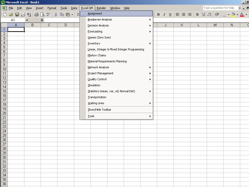
142. We Scroll To The “ ASSIGNMENT “ Module

143. We Want To Solve A New Problem

144. The Dialog Box Appears

145. There Are Four ( 4 ) Jobs To Be Assigned There Are Four ( 4 ) Workers or Machines That Are Available The Objective Function Is To Minimize Total Time or Cost The Jobs Are Labeled A, B, C, etc.

146. The Workers Are Numbered As 1, 2, 3, 4

147. THE DATA INPUT TABLE

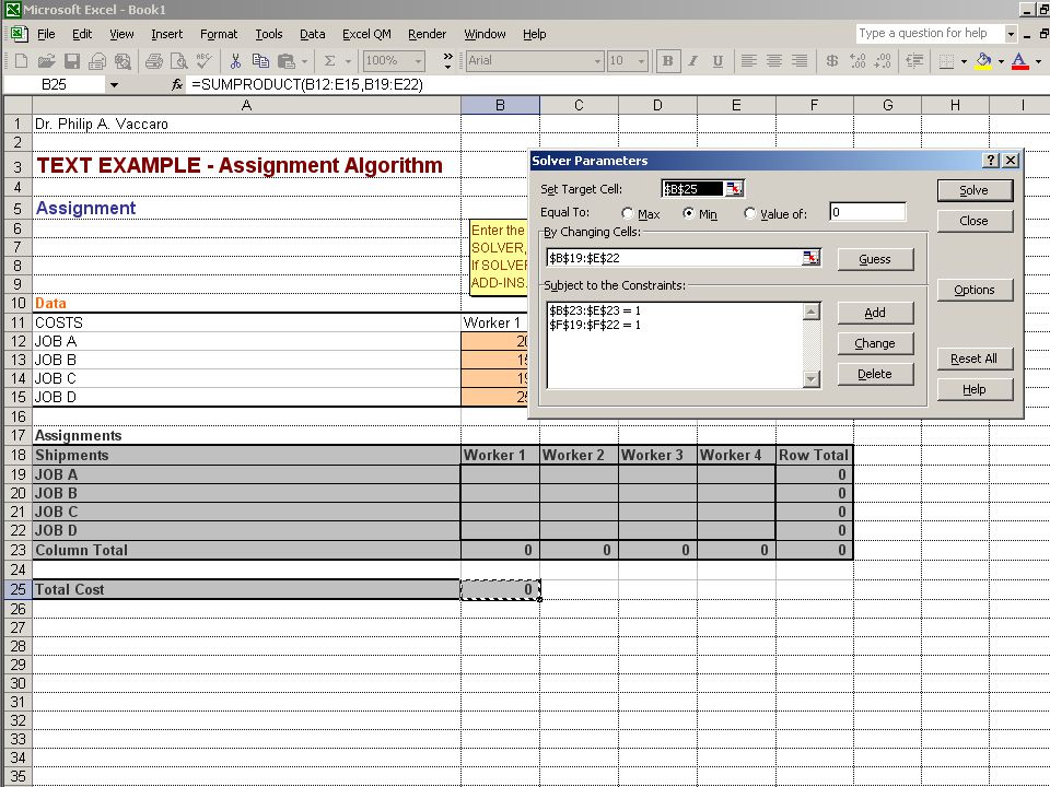
148. THE COMPLETED DATA INPUT TABLE INCLUDES THE COST OF PROCESSING EACH JOB BY EACH WORKER

149. THE OPTIMAL SOLUTION Assign Worker 1 to Job A Assign Worker 2 to Job C Assign Worker 3 to Job D Assign Worker 4 to Job B Total Minimum Cost = $78.00

151. THE “ TILE “ OPTION all solution windows can be displayed simultaneously and removed one by one after discussion

152. THE “CASCADE” OPTION All window solutions can be discussed and removed one by one afterwards

153. The Assignment Algorithm Assignment Algorithm

156. Template and Sample Data

162. The Assignment Algorithm Applied Management Science for Decision Making, 1e © 2012 Pearson Prentice-Hall, Inc. Philip A. Vaccaro, PhD