1. Decision Theory Lecture 8

2. 1/3 1 1/4 3/8 1/4 3/8 A A B C A B C 1/2 A B A C Reduction of compound lotteries 1/2 1/4 A B C

3. Von Neumann Morgenstern proof graphically 1

4. Von Neumann Morgenstern proof graphically 2

5. Common misunderstandings

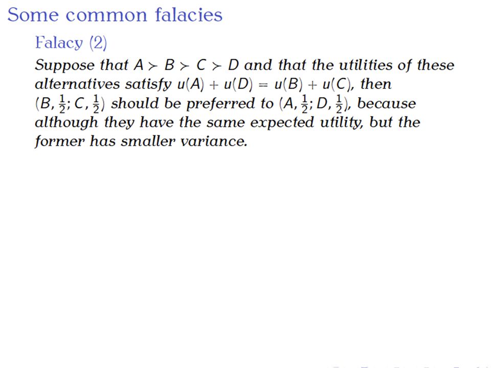
7. Fallacy (2) Fire insurance: – Fire: pay the premium, house rebuilt (C) – No Fire: pay the premium, house untouched (B) No insurance: – Fire: house burnt, no compansation (D) – No Fire: house the same (A) A≻B≻C≻D Suppose the probability of fire is 0.5 And an individual is indifferent between buying and not buying the insurance Although Fire insurance has smaller variance and ½u(A) + ½u(D) = ½u(B) + ½u(C), it does not mean that Fire insurance should be chosen over No insurance Loss = $70K Loss = $60K Loss = $K Loss = $0 Risk averse, and EL(insurance) = $65K EL(no insurance) = $50K

8. Fallacy (3) Fire insurance: – Fire: pay the premium, house rebuilt (C) – No Fire: pay the premium, house untouched (B) No insurance: – Fire: house burnt, no compansation (D) – No Fire: house the same (A) A≻B≻C≻D Suppose that the probability of fire is ½ and an individual prefers not buying fire insurance and hence ½u(A) + ½u(D) > ½u(B) + ½u(C) ⇒ u(A) - u(B) > u(C) - u(D) However it does not mean that the change from B to A is more preferred than the change from D to C. Preferences are defined over pairs of alternatives not pairs of pairs of alternatives

13. Crucial axiom - independence Our version The general version Why the general version implies our version?

14. If I prefer to go to the movies than to go for a swim, I must prefer: – to toss a coin and: heads: go to the movies tails: vacuum clean – than to toss a coin and: heads: go for a swim tails: vacuum clean If I prefer to bet on red than on even in roulette, then I must prefer: – to toss a coin and heads: bet on 18 tails: bet on red – than to toss a coin and: heads: bet on 18 tails: bet on even Independence – examples 14

15. Machina triangle 15 p1p1 p2p2 1 1 x2x2 x3x3 P R   x1x1  P +  R

16. Independence assumption in the Machina triangle 16 p1p1 p2p2 1 1 P Q R αP+(1-α)R αQ+(1-α)R Suppose that A1 is better than A2 is better than A3

17. 17.1 and 17.2 17.1) Choose one lottery: P=(1 mln, 1) Q=(5 mln, 0.1; 1 mln, 0.89; 0 mln, 0.01) 17.2) Choose one lottery: P’=(1 mln, 0.11; 0 mln, 0.89) Q’=(5 mln, 0.1; 0 mln, 0.9) Kahneman, Tversky (1979) [common consequence effect violation of independence] Many people choose P over Q and Q’ over P’

18. Common consequence graphically P = (1 mln, 1) P’= (1 mln, 0.11; 0, 0.89) Q = (5 mln, 0.1; 1 mln, 0.89; 0, 0.01) Q’= (5 mln, 0.1; 0, 0.9) If we plug c = 1mln, we get P and Q respectively If we plug c = 0, we get P’ and Q’ respectively

19. 18.1 i 18.2 18.1) Choose one lottery: P=(3000 PLN, 1) Q=(4000 PLN, 0.8; 0 PLN, 0.2) 18.2) Choose one lottery: P’=(3000 PLN, 0.25; 0 PLN, 0.75) Q’=(4000 PLN, 0.2; 0 PLN, 0.8) Kahneman, Tversky (1979) [common ratio effect, violation of independence] Many people choose P over Q and Q’ over P’

20. Common ratio graphically P=(3000 PLN, 1) P’=(3000 PLN, 0.25; 0 PLN, 0.75) Q=(4000 PLN, 0.8; 0 PLN, 0.2) Q’=(4000 PLN, 0.2; 0 PLN, 0.8)

21. Monotonicity of utility function BehaviourPrefers more to less 21 x x+ 

22. Monotonicity of utility function BehaviourPrefers more to less Utility function  x, u’(x)>0; u(x) – increasing 22

23. Monotonicity of utility function BehaviourPrefers more to less Utility function  x, u’(x)>0; u(x) – increasing Attitude towards risk (quantitatively)u(x)/u’(x) – fear of ruin 23 prefers more to less current wealth x probability p of bankruptcy (u(0)=0) how much to pay to avoid it?

24. Monotonicity of utility function BehaviourPrefers more to less Utility function  x, u’(x)>0; u(x) – increasing Attitude towards risk (quantitatively)u(x)/u’(x) – fear of ruin When is the choice obvious First order stochastic dominance (comparing cdf) – FOSD 24 F(x) 1 x

25. Examples – comparing pairs of lotteries PayoffPr. 150% 230% 320% PayoffPr. 410% 550% 640% PayoffPr. 150% 230% 320% PayoffPr. 140% 230% 3 PayoffPr. 150% 230% 320% PayoffPr. 250% 330% 420% PayoffPr. 150% 230% 320% PayoffPr. 140% 235% 325%

26. First Order Stochastic Dominance (FOSD) PayoffPr. 150% 230% 320% PayoffPr. 410% 550% 640% t cdf 1 1 PayoffPr. 150% 230% 320% PayoffPr. 140% 235% 325% t cdf 1 1

27. FOSD Assume X and Y are two different lotteries (F X (.), F Y (.) are not the same) Lottery X FOSD Y if: For all a, hence: Those who prefer more to less will never choose lottery that is dominated in the above sense. Theorem: X FOSD Y if and only if Eu(X) ≥ Eu(Y), for all inreasing u

28. Compare PayoffPr. 150% 230% 320% PayoffPr. 140% 250% 310% PayoffPr. 150% 230% 320% PayoffPr. 140% 230% 3 PayoffPr. 150% 230% 320% PayoffPr. 290% 35% 4 PayoffPr. 110% 270% 320% PayoffPr. 030% 255% 415%

29. Marginal utility Behaviour Risk averse, ie. Var(L)>0  u(E(L))>E(u(L)) 29 x x-  x+  Today chance nodes split 50:50

30. Marginal utility Behaviour Risk averse, ie. Var(L)>0  u(E(L))>E(u(L)) Utility function  x, u’(x)>0, u’’(x)<0; u(x) – concave, increasing 30 payoff utility

31. Certainty equivalent and risk premium  0,5 2 10 1 4,5 1 6 utility

32. Marginal utility Behaviour Risk averse, ie. Var(L)>0  u(E(L))>E(u(L)) Utility function  x, u’(x)>0, u’’(x)<0; u(x) – concave, increasing Attitude towards risk (quantitatively)-u’’(x)/u’(x) – Arrow-Pratt risk aversion coeff. 32 x – initial wealth (number) l – lottery with zero exp. value (random variable) k – multiplier (we tak k close to zero) d – risk premium (number) x-d – certainty equivalent for x+l

33. Marginal utility Behaviour Risk averse, ie. Var(L)>0  u(E(L))>E(u(L)) Utility function  x, u’(x)>0, u’’(x)<0; u(x) – concave, increasing Attitude towards risk (quantitatively)-u’’(x)/u’(x) – Arrow-Pratt risk aversion coeff. When is the choice obvious Second order stochastic dominance (integrals of cdf) – SOSD 33

34. Second Order Stochastic Dominance PayoffPr. 150% 220% 330% PayoffPr. 130% 260% 310% t cdf 1 1 t 1 1 tF(x)Sum 10,30 20,90,3 311,2 412,2 tF(x)Sum 10,50 20,70,5 311,2 412,2

35. SOSD Assume X and Y are two different lotteries (F X (.), F Y (.) are not the same) Lottery X SOSD Y if: For all a hence: Those who are risk averse will never choose a lottery that is dominated in the above sense. Theorem: X SOSD Y if and only if Eu(X) ≥ Eu(Y), for all inreasing and concave u

36. Compare and find FOSD and SOSD PayoffPr. 130% 240% 330% PayoffPr. 140% 215% 345% PayoffPr. 150% 230% 320% PayoffPr. 160% 210% 330% PayoffPr. 110% 250% 340% PayoffPr. 130% 215% 355% PayoffPr. 115% 245% 340% PayoffPr. 120% 240% 3

37. Risk aversion doesn’t mean that always: A better than B, if only E(A)=E(B) and Var(A)<Var(B) – some lotteries do not result from another with mean preserving spread – is true when Var(A)=0 Mean-variance criterium works e.g. for normally distributed random variables (lotteries) Mean-variance criterium 37 Lottery XLottery Y Prob.xu(x)=ln(x)(x-EX) 2 yu(y)=ln(y)(y-EY) 2 20%20,1365,6141,38664 80%9,9752,34,1142,6394 mean122,4416,4122,38816

38. Measures of risk aversion Risk premium measures risk aversion with respect to a given lottery As a function of payoff values risk aversion is measured by Arrow, Pratt measures of (local) risk aversion

39. From now on let’s assume X is a set of monetary pay- offs (decision maker prefers more money than less) Decision maker with vNM utility function prefers lottery (100, ¼; 1000, ¾) to (500, ½; 1000, ½) What is a realtion between (100, ½; 500, ¼; 1000, ¼) and (100, ¼; 500, ¾)? Suggestion – we can arbitrarily set utility function for two outcomes Exercise 1 39

40. Decision maker is indifferent between pairs of lotteries: (500, 1) and (0, 0,4; 1000, 0,6) and (300, 1) and (0, ½; 500, ½) Can we guess the preference relation between (0, 0,2; 300, 0,3; 1000, ½) and (500, 1)? Exercise 2 40

41. Decision maker with vNM utility is risk averse and indifferent between the following pairs (400, 1) and (0, 0,3; 1000, 0,7) and (0, ½; 200, ½) and (0, 5/7; 400, 2/7) Can we guess the preference relation between (200, ½; 600, ½) and (0, 4/9; 100, 5/9)? (suggestion – remamber than vNM utility is concave) Exercise 3 41