1. 8. Failure Rate Prediction Reliable System Design 2011 by: Amir M. Rahmani

2. matlab1.ir Bathtub Curve Three phases of system lifetime – Infant mortality – Normal lifetime – Wear-out period Every product has a failure rate, λ which is the number of units failing per unit time.

3. Bathtub Curve (2) It is the manufacturer’s aim to ensure that product in the Infant mortality period does not get to the customer. This leaves a product with a Normal lifetime period during which failures occur randomly i.e. λ is constant, and finally a Wear-out period, usually beyond the products Normal lifetime, where λ is increasing. matlab1.ir

4. Usefulness of failure rate prediction - to assess whether reliability goals can be reached, - to identify potential design weaknesses, - to compare alternative designs, - to evaluate designs and to analyze life-cycle costs, - to provide data for system reliability and availability analysis, - to plan logistic support strategies, - to establish objectives for reliability tests. matlab1.ir

5. The failure rate prediction process - define the equipment to be analyzed - understand system by analyzing equipment structure - determine operational conditions: operating temperature, rated stress; - determine the actual electrical stresses for each component; - extract the reference failure rate for each component from the database; - sum up the component failure rates; - document the results and the assumptions. matlab1.ir

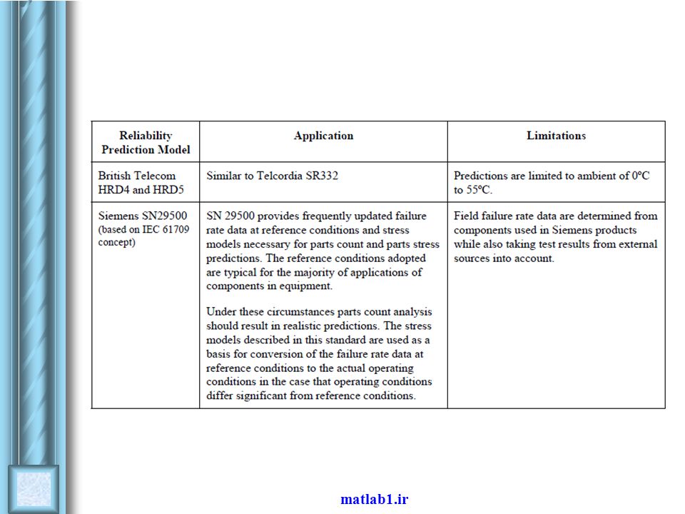
6. Failure Rate Calculation How do we can calculate failure rate? - Experimental system observation Needs to very long time Technology wear-out High cost - Failure prediction with standards Telcordia SR332/ Bellcore TR332 British Telecom HRD4 and HRD5 Siemens SN29500 (based on IEC 61709

7. COMPARISON OF FEATURES OF RELIABILITY PREDICTION METHODS matlab1.ir

9. Failure Rate Prediction Mil-Hdbk-217F, 217F_1, 217F_2 Microprocessor, PAL, PLA, MOS device λ p = Π L Π Q (C 1 Π T + C 2 Π E ) failures/10 6 hours λ p is the part failure rate Π L represents the learning factor and is determined by the experience of the manufacturer Π Q is determined by the part quality C 1 is related to die complexity Π T is related to ambient temperature C 2 is related to the package type Π E is determined by the operating environment

10. matlab1.ir Failure Rate Prediction Π L : learning factor (section 5.10) Π L =2, for a new chip Π L =1 for product of a chip with high experience Π L = 0.01exp(5.35-0.35*year) Π Q : quality factor, chips testing before selling (section 5.10) 1- A: Π Q =1, high quality military application (all chips will be tested) 2- B: Π Q =2, military application 3- C: Π Q =16, high quality commercial application (e.g. one of 1000 chips will be tested) 4- D: Π Q =150, standard components

11. matlab1.ir Failure Rate Prediction Π T : temperature factor (section 5.8) depends on: Device technology Packaging type Case temperature Power dissipation Π T = 0.1e -A(1/(Tj+273) – 1/298) A depends on: –Device technology –Packaging type T j = T c + θ jc * P –T c is case temperature –θ jc is temperature resistance between case and junctions –P is Max. of power dissipation

12. matlab1.ir Failure Rate Prediction C 1 : Die complexity (section 5.1) Microprocessor C 2 : Package type (section 5.9) for hermetic DIP C 2 = 2.8 * 10 -4 (N p ) 1.08 N p = Number of functional pin Π E : environment factor, (section 5.10), Table 3-2 Number of bitsBipolarCMOS Up to 80.060.14 Up to 160.120.28 Up to 320.240.56

13. matlab1.ir Failure Rate Prediction: Example What is the failure rate of MC6800 microprocessor? What is the failure rate for each gate? What is the MTTF? Function: 8-bit processor No. of gate:12667 Number of pins64 Technology:NCMOS Packaging:64 pin ceramic DIP hermetically Power dissipation:1.5 W Environment:room Case temperature:35 oc Power supply:+5 v Quality:commercial

14. matlab1.ir Failure Rate Prediction: Example Π L = 1, Π Q = 150 Π T = 0.1*e -5794(1/(35+15*1.5+273)-1/298) = 0.68 C 1 = 0.06 C 2 = 2.8* (10 -4 )*(64) 1.08 = 0.025 Π E = 0.38 λ CPU =Π L Π Q (C 1 Π T +C 2 Π E )= 0.75*10 -6 failures/hour λ gate = λ CPU /12667 = 0.395*10 -10 failures/hour MTTF = 1/λ = 1/0.5*10 -6 = 2*10 6 ≈ 228 years

15. matlab1.ir Failure Rate Prediction Mil-Hdbk-217F Memories, SRAM, DRAM, xROM λ p = Π L Π Q (C 1 Π T + C 2 Π E +λ cyc ) failures/10 6 hours λ p is the part failure rate Π L represents the learning factor and is determined by the experience of the manufacturer Π Q is determined by the part quality C 1 is related to die complexity Π T is related to ambient temperature C 2 is related to the package type Π E is determined by the operating environment

16. matlab1.ir Hardware failure rates Ways of improving reliability of hardware – Decrease temperature – Decrease electrical stress – Reduce number of components or increase integration – Increase quality of components – Improve physical environment