Download presentation
Presentation is loading. Please wait.

1
Image Reconstruction and Inverse Treatment Planning – Sharpening the Edge – Thomas Bortfeld I.CT Image Reconstruction II.Inverse Treatment Planning

2
2 Syllabus 2/13Advances in imaging for therapy (Chen) 2/20Treatment with protons and heavier particles; tour of proton facility (Kooy) 2/27Treatment delivery techniques with photons, electrons; tour of photon clinic (Biggs, Folkert) 3/6Intensity-modulated radiation therapy (IMRT, IMPT) (Seco, Trofimov) 3/13Dose calculation (Monte Carlo + otherwise) (Paganetti, Kooy) 3/20Treatment planning (photons, IMRT, protons) (Doppke + NN)
 2/20Treatment with protons and heavier particles; tour of proton facility (Kooy) 2/27Treatment delivery techniques with photons, electrons; tour of photon clinic (Biggs, Folkert) 3/6Intensity-modulated radiation therapy (IMRT, IMPT) (Seco, Trofimov) 3/13Dose calculation (Monte Carlo + otherwise) (Paganetti, Kooy) 3/20Treatment planning (photons, IMRT, protons) (Doppke + NN)")
3
3 Syllabus 3/27Inverse treatment planning and optimization (Bortfeld) 4/3Optimization with motion and uncertainties (Trofimov, Unkelbach) 4/10Mathematics of multi-objective optimization and robust optimization (Craft, Chan) 4/17Dose painting (Grosu) 4/24Image-guided radiation therapy (Sharp) 5/1Special treatment techniques for moving targets (Engelsman)
 4/3Optimization with motion and uncertainties (Trofimov, Unkelbach) 4/10Mathematics of multi-objective optimization and robust optimization (Craft, Chan) 4/17Dose painting (Grosu) 4/24Image-guided radiation therapy (Sharp) 5/1Special treatment techniques for moving targets (Engelsman)")
4
4 Planigraphy, Tomosynthesis “Verwischungstomographie” Ziedses des Plantes (Netherlands), 1932 x-ray source focus slice x-ray tube object film
, 1932 x-ray source focus slice x-ray tube object film")
5
5 Computerized Tomography Greek: tomos = section, slice graphia = to write, to draw tomograph = slice drawer

6
6 Nobel prize 1979 Drs. Hounsfield and Cormack Sir Godfrey N. Hounsfield (Electrical Engineer) EMI Allan M. Cormack (Physicist) South Africa, Boston
 EMI Allan M. Cormack (Physicist) South Africa, Boston.")
7
7 First CT scanner prototype Hounsfield apparatus

8
8 CT “generations” 1 st generation2 nd generation translation-rotation scanners

9
9 CT “generations” 3 rd generation (fan detector) Rotation-only scanners 4 th generation (ring detector)
 Rotation-only scanners 4 th generation (ring detector)")
10
10 Imatron: Electron beam CT (EBT)
")
11
11 Imatron: Electron beam CT (EBT)
")
12
12 Helical (“spiral”) CT Start of spiral scan Trajectory of the continuously rotating X-ray tube Table motion
 CT Start of spiral scan Trajectory of the continuously rotating X-ray tube Table motion")
13
13 From transmission to projection A.M. Cormack

14
14 Projection

15
15 Sinogram, “Radon” transform, Johann Radon, Vienna, 1917) Object p Sinogram p ?
 Object p Sinogram p ")
16
16 Backprojection

17
17 Backprojection Shepp&Logan phantom“Reconstruction” by backprojection

18
18 Backprojection

19
19 Projections of point object from three directions Back-projection onto reconstruction plane Backprojection

20
20 Backprojection Profile through objectProfile through image Object f(r) Image f(r) 1/r Terry Peters (Robarts Institute)
 Image f(r) 1/r Terry Peters (Robarts Institute)")
21
21 Backprojection This is a convolution (f * h) of f(r) with the point spread function (PSF) h=1/|r|
 of f(r) with the point spread function (PSF) h=1/|r|")
22
22 What is Convolution?

23
23 Convolution theorem Periodic sine-like functions are the Eigenfunctions of the convolution operation. This means, convolution changes the amplitude of a sine wave but nothing else. Hence, convolution is completely described by the transfer function or frequency response (Fourier transform of the PSF), which determines how much amplitude is transmitted for different frequencies
, which determines how much amplitude is transmitted for different frequencies.")
24
24 Convolution theorem

25
25 -filtered layergram reconstruction 1.Backproject measured projections, and integrate over 2.Fourier transform in 2D 3.Multiply with distance from the origin, | |, in the frequency space 4.Inverse Fourier transform

26
Central slice theorem

27
27 Filtered backprojection

28
28 Deconvolution (filtering) in the spatial domain Ramp filter in the frequency domain: Transform back to get filter in spatial domain: sampling interval
 in the spatial domain Ramp filter in the frequency domain: Transform back to get filter in spatial domain: sampling interval")
29
29 Deconvolution (filtering) in the spatial domain Sample at discrete points p = n p: sampling interval Filter of Ramachandran and Lakshminarayanan (Ram-Lak)
 in the spatial domain Sample at discrete points p = n p: sampling interval Filter of Ramachandran and Lakshminarayanan (Ram-Lak)")
30
30 Ram-Lak filter negative components

31
31 Shepp&Logan filter

32
32 Backprojecting filtered projections Terry Peters (Robarts Institute)
")
33
33 Filtered backprojection Shepp&Logan phantom“Reconstruction” by backprojectionFiltered backprojection

34
34 Filtered Backprojection Simple backprojectionFiltered backprojection

35
35 Reconstruction from fan projections k: counter of source positions l: counter of projection lines k+l = 7: parallel

36
36 Summary CT image reconstruction 1.In CT we measure projections, i.e., line integrals 2.The set of projection lines from all directions is called Radon transform or sinogram 3.Backprojection leads back into image space but introduces severe 1/r blurring

37
37 Summary CT image reconstruction, cont’d 4.Image can be de-blurred with deconvolution techniques 5.Deconvolution can be done in projection space using the central slice theorem 6.A common filter function is the Ram-Lak filter 7.Filters have negative components (“eraser”) to remove blurring
 to remove blurring")
38
Image Reconstruction and Inverse Treatment Planning – Sharpening the Edge – Thomas Bortfeld I.CT Image Reconstruction II.Inverse Treatment Planning

40
40 Phantom Target OAR Dose Source Brahme, Roos, Lax 1982

41
41 The idea of IMRT Treated Volume Tumor OAR Target Volume Intensity Modulation Treated Volume OAR Target Volume Collimator "Classical" Conformation

42
42 “Inverse” treatment planning Treated Volume OAR Target Volume Collimator Treated Volume OAR Target Volume Inverse Planning"Conventional" Planning

43
Conformal RadiotherapyComputer Tomography Intensity Modulation Target Projection Detectors Radiation Source Radiation Source

44
44 Image Reconstruction (Filtered Backprojection) Conformal Radiotherapy (Filtered Projection) x-ray Projection (CT-Scanner) x-ray Projection (CT-Scanner) IMRT with Filtered Projections IMRT with Filtered Projections Projection (Computer) Projection (Computer) 1D Filtering of the Projections 1D Filtering of the Projections Backprojection 1D Filtering of the Projections 1D Filtering of the Projections Density Distribution of the Tissue Set of Prescribed 2D Dose Distributions Dose DistributionSet of 2D Slice Images
 Conformal Radiotherapy (Filtered Projection) x-ray Projection (CT-Scanner) x-ray Projection (CT-Scanner) IMRT with Filtered Projections IMRT with Filtered Projections Projection (Computer) Projection (Computer) 1D Filtering of the Projections 1D Filtering of the Projections Backprojection 1D Filtering of the Projections 1D Filtering of the Projections Density Distribution of the Tissue Set of Prescribed 2D Dose Distributions Dose DistributionSet of 2D Slice Images")
45
G. Birkhoff: On drawings composed of uniform straight lines Journ. de Math., tome XIX, - Fasc. 3, 1940.

46
46 After filtering: x Intensity Negative Intensities -

47
Consider the inverse problem as an optimization problem. Define the objectives of the treatment and let the computer determine the parameters giving optimal results. The inverse problem has no solution!

48
Objective Function F(x) = i (d i - p i ) 2, d i = f(x 1,.., x n ) F(x) = NTCP (1-TCP) Constraints d i 0 DVH constraints NTCP < 5% Parameters x = (x 1,..., x n ) (e.g., intensity values) Mathematical optimization: Minimization of objective functions actual doseprescribed dose Optimization basics
 = i (d i - p i ) 2, d i = f(x 1,.., x n ) F(x) = NTCP (1-TCP) Constraints d i 0 DVH constraints NTCP < 5% Parameters x = (x 1,..., x n ) (e.g., intensity values) Mathematical optimization: Minimization of objective functions actual doseprescribed dose Optimization basics")
49
“Decision variables” Intensity profiles Beam weights, segment weights Beam angles (gantry angle, table angle) Number of beams Energy (especially in charged particle therapy) Type of radiation (photons, electrons,...)
 Number of beams Energy (especially in charged particle therapy) Type of radiation (photons, electrons,...)")
50
50 The “standard model” of inverse planning : dose contribution of pencil beam j to voxel i all the physics is here beam intensities dose values minimize

51
small weight (w) Volume DoseD max large weight (w) DVH Volume D max Dose DVH Dose-volume histogram for OAR
 Volume DoseD max large weight (w) DVH Volume D max Dose DVH Dose-volume histogram for OAR")
52
52 Critical structure (organ at risk) costlet weight importance “penalty” dose at voxel i in OAR k tolerance dose
 costlet weight importance penalty dose at voxel i in OAR k tolerance dose")
53
Volume Dose DVH D max D min Dose-volume histogram for the target

54
54 The “standard model” of inverse planning Minimize weights, penalties, importance factors objectives, costlets, indicators

55
55 The “standard model” of inverse planning High-dimensional problem: Ray intensities b j : 10,000 Dose voxels d i : 500,000 D ij matrix: 10,000 x 500,000 entries 20 GByte

56
56 x1x1 x0x0 x3x3 x F(x) local min. global min. 1D: Optimization with gradient descent x2x2
 local min. global min. 1D: Optimization with gradient descent x2x2")
57
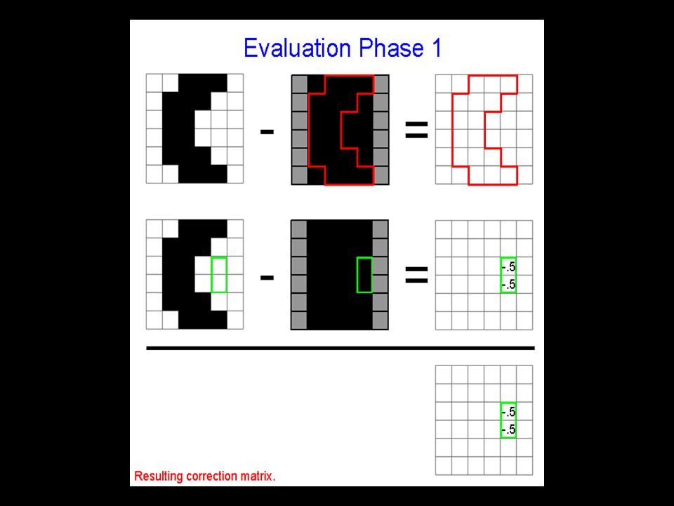
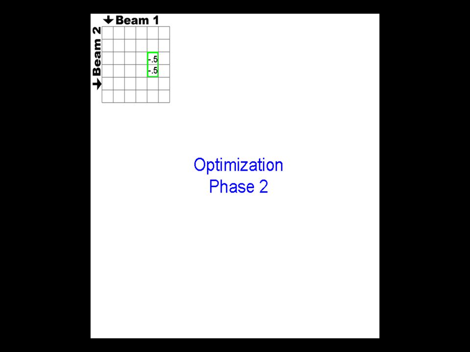
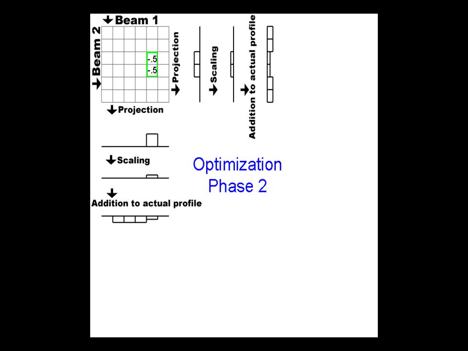
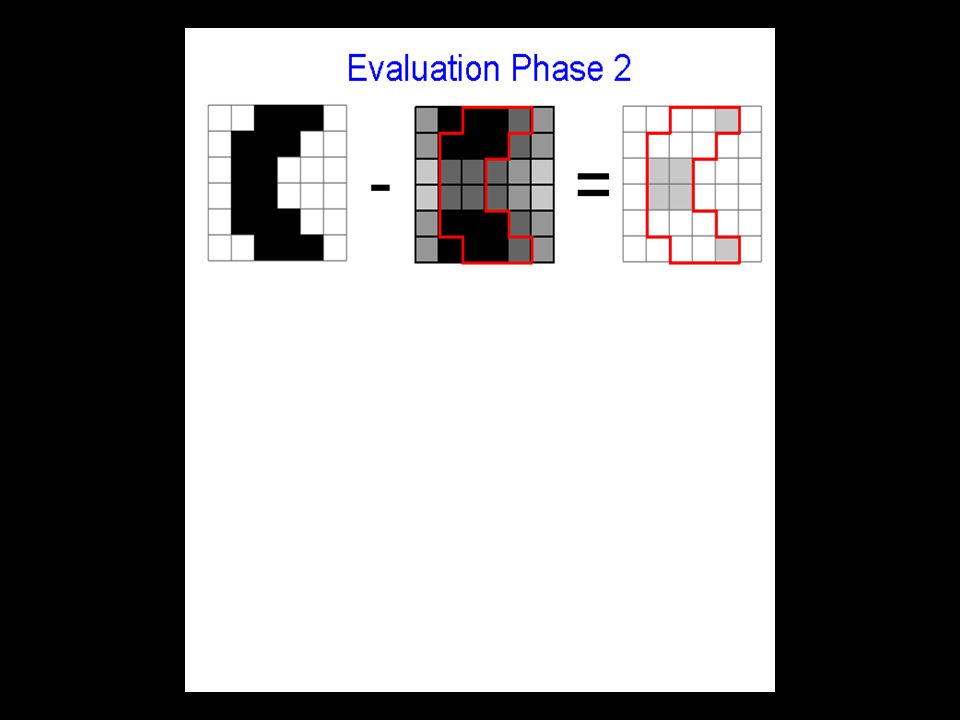
57 Optimization algorithms Projecting back and forth between dose distribution and intensity maps

78
78 Volume effect Whole lung: 18 Gy 50% of lung: 35 Gy

79
79 Volume effect Power-law relationship for tolerance dose (TD): n small: small “volume effect” n large: large “volume effect”
: n small: small volume effect n large: large volume effect")
80
80 Volume effect -> EUD, Power-Law (a-norm) Model “a-norm” (a=1/n) Mohan et al., Med. Phys. 19(4), 933-944, 1992 Kwa et al., Radiother. Oncol. 48(1), 61-69, 1998 Niemierko, Med. Phys. 26(6), 1100, 1999 Examples:
, , 1992 Kwa et al., Radiother. Oncol. 48(1), 61-69, 1998 Niemierko, Med. Phys. 26(6), 1100, 1999 Examples:.")
81
81 0 25 50 75 100 0204060 Volume [%] Dose [Gy] 80 100 EUD = The homogeneous dose that gives the same clinical effect Lung: EUD = 25 Gy Spinal Cord: EUD = 52 Gy Equivalent Uniform Dose (EUD)
![Volume [%] Dose [Gy] EUD = The homogeneous dose that gives the same clinical effect Lung: EUD = 25 Gy Spinal Cord: EUD = 52 Gy Equivalent Uniform Dose (EUD)](http://images.slideplayer.com/13/3894146/slides/slide_81.jpg "Volume [%] Dose [Gy] EUD = The homogeneous dose that gives the same clinical effect Lung: EUD = 25 Gy Spinal Cord: EUD = 52 Gy Equivalent Uniform Dose (EUD)")
82
82 DVH constraint Volume Dose D max V

83
83 Dose, Dose-Volume Constraints Penalties/ Weights/ …

84
84 Summary inverse treatment planning 1.Intensity-modulated radiation therapy (IMRT) uses non-uniform beam intensities from various (5-9) beam directions 2.“Inverse planning” is the calculation of intensities that will give the desired spatial dose distribution 3.CT reconstruction techniques cannot be (directly) applied here because we cannot deliver negative intensities 4.Today “inverse planning” is usually defined as an optimization problem, which is “solved” with gradient techniques
 uses non-uniform beam intensities from various (5-9) beam directions 2. Inverse planning is the calculation of intensities that will give the desired spatial dose distribution 3.CT reconstruction techniques cannot be (directly) applied here because we cannot deliver negative intensities 4.Today inverse planning is usually defined as an optimization problem, which is solved with gradient techniques")
Similar presentations


 of radiation directed toward the pt. and the remnant radiation emitted from the pt.>")

 Algorithm.>")


 Computer tomography (CT) Proton therapy Electrical impedance.>")


