1. KRUSKAL-WALIS ANOVA BY RANK (Nonparametric test)
this non-parametric test makes no assumptions about the distribution of the data (e.g., normality)
More than 2 groups – a nonparametric alternative to the one way ANOVA.
Median of >3 groups are tested
It uses the ranks of the data rather than their raw values to calculate the statistic
Definition
A non-parametric test (distribution-free) used to compare three or more independent groups of sampled data.

2. Steps of Kruskal-Walis Test
All observations from k samples (k groups) are combined into a single series and arranged in order magnitude from smallest to largest.
The observations are then replaced by ranks. The smallest observation is replaced by rank 1, the next to smallest by rank 2 and the largest by rank N.
The sum of the ranks in each sample (column) is taken.
The Kruskal-Walis Test determines whether these sums of ranks are so disparate that they are not likely to come from same population or not.
H value is compared to a table of critical values for U based on the sample size of each group. If H exceeds the critical value for H at some significance level (usually 0.05) it means that there is evidence to reject the null hypothesis in favor of the alternative hypothesis.

3. Steps of Kruskal-Walis Test
The test statistic
Where k = number of sample
n = number of observations in each group.
N = the number of observations in all samples combined.
R = sum of ranks in in each group

4. Example:
The effects of 2 drugs on reaction time to a certain stimulus were studied in 3 groups of experimental animals. Group 3 served as a control and other two groups were treated by drug A & B.
Data from 3 independent groups are given in the table
Group A
Group B 17 8 20 7 40 9 31 35
Group C 2 5 4 3
Data (in ascending order, from all groups):
Rank:

5. Example: Ranks from 3 groups are given in the table
Group A
Group B
Group C 9
6.5 1 10 5 4 13 8 3 11 2 12
R1 = 55
R2 = 26
R 3= 10
This value is compared to a table of critical values for H based.
Table shows that when the nj are 5, 4 and 4, calculated H is more than table value (>10.68) at p< The null hypothesis is rejected at the 0.01 level of significance.
Conclusion: We conclude that there is a difference in the average reaction time among the three groups.

6. Adjustment for Tied values
Since the values of H is somewhat influenced by ties, H is corrected
/adjusted by dividing it by
Where T = t3 – t (when t is the number of tied observations in a group of tied values) and
N = number of observation in all k groups together, that is,
Therefore H corrected for ties is

7. Adjustment for Tied values
Since there were 2 tied values in our group of ties, we have T = 23 – 2 = 6 and Therefore,
Therefore H corrected for ties is

8. KRUSKAL-WALIS TEST
The results of this test indicate that there is a significant difference or not between groups.
The Tukey multiple comparisons are used to specify which groups differ.

9. Spearman Rank Correlation Coefficient
The conventional correlation coefficient (Pearson’s correlation coefficient) assumes that two variables being measured jointly follows Normal distribution.
Nonparametric measures of correlation (distribution free) is Spearman’s rank correlation coefficient.
Spearman’s rank correlation coefficient is calculated from ranks rather than from the original observations.
The x and y variables to be correlated are each ranked separately from smallest to biggest and then the rankings are correlated with one another.
It is designated by rs.

10. Steps Of Spearman Rank Correlation Coefficient
First rank the values fro low to higher.
Find the difference (di) between the ranks of Xi and the ranks of Yi.
Square each di and find the sum of the squared values (di2).
Compute

11. Steps of Spearman Rank Correlation Coefficient
For testing significance of rs, compute z value
Taking ties into account, correction is necessary. However, unless a substantial number of ties are involved, the resulting modifications are minor and, for all practical purposes, can be ignored.
Compare calculated value with table value to find p value. If p<0.05, the relation is significant.

12. Example
The following are the numbers of hours which 10 students studied for an examination and the grades which they received:
No of hours studied Grade in exam

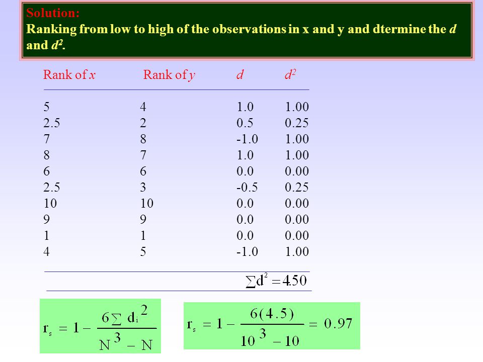
13. Solution:
Ranking from low to high of the observations in x and y and dtermine the d and d2.
Rank of x Rank of y d d2

14. For rs = 0.97 and n = 10, we get z value is
Solution: Test of significance of rs
The null hypothesis is there is no correlation, H0 : rs=0
For rs = 0.97 and n = 10, we get z value is
Since z = 2.91 exceeds (table value), the null hypothesis must be rejected at 0.01 level of significance, we conclude that there is a relationship between study time and grades of the students.

15. Odds ratio
In epidemiology, odds ratio are often used to measure the strength of the association between a risk factor and the disease.
This parameter should only be calculated if the chi-square test indicate that there is a relationship between the exposure and disease.
Odds ratio is used in case-control studies in which there is a group of diseased people (cases) and a group of undiseased people (control).
The odds is defined as the ratio of the probability of an event (disease) happening over the chance that will no happen.
The odds ratio then becomes the ratio of the odds in the exposed group over the odds in the unexposed group.
Case control study
Disease present Disease absent
Exposed a b
Unexposed c d
Odds of disease in the exposed group is a/b and in the unexposed group is c/d.
The odds ratio is then,

16. Odds ratio MI case Control Alcohol 71 52 No alcohol 29 48
Confidence interval for odds ratio is:
Example: The following data from a case-control study of myocardial infarction (MI) and alcohol intake
Does this suggest that there is an association between disease and alcohol consumption?
MI case Control
Alcohol
No alcohol
CI: – 4.06
The interval does not include 1. With 95% CI, the true odds ratio lies
between 1.26 and Since this interval does not include null value 1, the observed association is statistically significant at 5% level.

17. Relative Risk (RR)
The risk of an event is the probability that an event will occur within a stated period of time.
It is the incidence rate of disease in the exposed group divided by the incidence of disease in the unexposed group is used only when you determined the number of people developing disease in each group over a period of time, i.e., in cohort or prospective studies.
The risk of developing the disease within the follow-up time is a/(a+b) for the exposed population and c/(c+d) for unexposed population.
Incidence (risk) in the exposed group: a/(a+b)
Risk in the unexposed: c/(c+d)
Relative risk =

18. Numbers of women in cohort study of serum ferritin and anemia
Relative Risk (RR)
Numbers of women in cohort study of serum ferritin and anemia
Anemia at 2nd survey
Not anemia at 2nd survey
Total
Serum ferritin <20mg 1st survey 7 8 15
Serum ferritin >20mg 1st survey 2 13
Relative risk =
= 7 x 15/(2 x 15) = 3.5.
Interpretation:
Here the relative risk, RR is 3.5. This is interpreted as a woman is 3.5 times more likely to become anemic if her serum ferritin is below 20 mg/l.

19. 95% Confidence interval for RR is: