1. Next Week The Vernal Equinox
Now on to Chapter 12: Measuring the Properties of Stars
When does the Spring Equinox Occur?

2. The Family of Stars
Those tiny glints of light in the night sky are in reality huge, dazzling balls of gas, many of which are vastly larger and brighter than the Sun
They look dim because of their vast distances
Astronomers cannot probe stars directly, and consequently must devise indirect methods to ascertain their intrinsic properties
Measuring distances to stars and galaxies is not easy
Distance is very important for determining the intrinsic properties of astronomical objects

3. Triangulation
Measure length of a triangle’s “baseline” and the angles from the ends of this baseline to a distant object
Use trigonometry or a scaled drawing to determine distance to object
Fundamental method for measuring distances to nearby stars is triangulation:

4. Trigonometric Parallax

5. Calculating Distance Using Parallax
A method of triangulation used by astronomers is called parallax:
Baseline is the Earth’s orbit radius (1 AU)
Angles measured with respect to very distant stars

6. Calculating Distance Using Parallax
The shift of nearby stars is small, so angles are measured in arc seconds
The parallax angle, p, is half the angular shift of the nearby star, and its distance in parsecs is given by:
dpc = 1/parc seconds
A parsec is 3.26 light-years (3.09 × 1013 km)
Useful only to distances of about 250 parsecs

7. Example: Distance to Sirius
Measured parallax angle for Sirius is arc second
From the formula,
dpc = 1/0.377
= 2.65 parsecs
= 8.6 light-years

8. The “Standard Candle” Method
If an object’s intrinsic brightness is known, its distance can be determined from its observed brightness
Astronomers call this method of distance determination the method of standard candles
This method is the principle manner in which astronomers determine distances in the universe
Intrinsic here refers to the properties of the star itself
Definition inserted

9. Light, the Astronomer’s Tool
Astronomers want to know the motions, sizes, colors, and structures of stars
This information helps to understand the nature of stars as well as their life cycle
The light from stars received at Earth is all that is available for this analysis

10. Temperature
The color of a star indicates its relative temperature – blue stars are hotter than red stars
More precisely, a star’s surface temperature (in Kelvin) is given by the wavelength in nanometers (nm) at which the star radiates most strongly

11. Luminosity
The amount of energy a star emits each second is its luminosity (usually abbreviated as L)
A typical unit of measurement for luminosity is the watt
Compare a 100-watt bulb to the Sun’s luminosity, 4 × 1026 watts

12. Luminosity
Luminosity is a measure of a star’s energy production (or hydrogen fuel consumption)
Knowing a star’s luminosity will allow a determination of a star’s distance and radius

13. The Inverse-Square Law
The inverse-square law relates an object’s luminosity to its distance and its apparent brightness (how bright it appears to us)

14. The Inverse-Square Law
This law can be thought of as the result of a fixed number of photons, spreading out evenly in all directions as they leave the source
The photons have to cross larger and larger concentric spherical shells.
For a given shell, the number of photons crossing it decreases per unit area

15. The Inverse-Square Law
The inverse-square law (IS) is:
B is the brightness at a distance d from a source of luminosity L
This relationship is called the inverse-square law because the distance appears in the denominator as a square

16. The Inverse-Square Law
The inverse-square law is one of the most important mathematical tools available to astronomers:
Given d from parallax measurements, a star’s L can be found (A star’s B can easily be measured by an electronic device, called a photometer, connected to a telescope.)
Or if L is known in advance, a star’s distance can be found

17. Radius
Common sense: Two objects of the same temperature but different sizes, the larger one radiates more energy than the smaller one
In stellar terms: a star of larger radius will have a higher luminosity than a smaller star at the same temperature

18. Knowing L “In Advance”
We first need to know how much energy is emitted per unit area of a surface held at a certain temperature
The Stefan-Boltzmann (SB) Law gives this:
Here s is the Stefan-Boltzmann constant (5.67 × 10-8 watts m-2K-4)

19. Tying It All Together
The Stefan-Boltzmann law only applies to stars, but not hot, low-density gases
We can combine SB and IS to get:
R is the radius of the star
Given L and T, we can then find a star’s radius!

20. Tying It All Together

21. Tying It All Together
The methods using the Stefan-Boltzmann law and interferometer observations show that stars differ enormously in radius
Some stars are hundreds of times larger than the Sun and are referred to as giants
Stars smaller than the giants are called dwarfs

22. Example: Measuring the Radius of Sirius
Solving for a star’s radius can be simplified if we apply L = 4pR2sT4 to both the star and the Sun, divide the two equations, and solve for radius:
Where s refers to the star and ¤ refers to the Sun
Given for Sirius Ls = 25L¤, Ts = 10,000 K, and for the Sun T¤= 6000 K, one finds Rs = 1.8R¤

23. The Magnitude Scale
About 150 B.C., the Greek astronomer Hipparchus measured apparent brightness of stars using units called magnitudes
Brightest stars had magnitude 1 and dimmest had magnitude 6
The system is still used today and units of measurement are called apparent magnitudes to emphasize how bright a star looks to an observer
A star’s apparent magnitude depends on the star’s luminosity and distance – a star may appear dim because it is very far away or it does not emit much energy

24. Magnitude Constellation Star 1 (Orion) Betelgeuse 2 Big Dipper various
(2) Astronomy Magazine Sept issue defines the faintest naked eye star at 6.5 apparent magnitude.
“Apparent Magnitude” was defined by Hipparachus in 150 BC. He devised a magnitude scale based on:
Magnitude Constellation Star
(Orion) Betelgeuse
Big Dipper various
stars just barely seen
However, he underestimated the magnitudes. Therefore, many very bright stars today have negative magnitudes.
Magnitude Difference is based on the idea that the difference between the magnitude of a first magnitude star to a 6th magnitude star is a factor of 100. Thus a 1st mag star is 100 times brighter than a 6th mag star. This represents a range of 5 so that = the fifth root of 100. Thus the table hierarchy is the following.
Absolute Magnitude is defined as how bright a star would appear if it were of certain apparent magnitude but only 10 parsecs distance.
Magnitude Difference of 1 is 2.512:1, 2 is :1 or 6.31:1, 3 is = 15.85:1 etc.

25. The Magnitude Scale The apparent magnitude can be confusing
Scale runs “backward”: high magnitude = low brightness
Modern calibrations of the scale create negative magnitudes
Magnitude differences equate to brightness ratios:
A difference of 5 magnitudes = a brightness ratio of 100
1 magnitude difference = brightness ratio of 1001/5=2.512

26. Images courtesy of Nick Strobel's Astronomy Notes
Images courtesy of Nick Strobel's Astronomy Notes. Go to his site at for the updated and corrected version.

27. The Magnitude Scale
Astronomers use absolute magnitude to measure a star’s luminosity
The absolute magnitude of a star is the apparent magnitude that same star would have at 10 parsecs
A comparison of absolute magnitudes is now a comparison of luminosities, no distance dependence
An absolute magnitude of 0 approximately equates to a luminosity of 100L¤

28. The Spectra of Stars
A star’s spectrum typically depicts the energy it emits at each wavelength
A spectrum also can reveal a star’s composition, temperature, luminosity, velocity in space, rotation speed, and other properties
On certain occasions, it may reveal mass and radius

29. Measuring a Star’s Composition
As light moves through the gas of a star’s surface layers, atoms absorb radiation at some wavelengths, creating dark absorption lines in the star’s spectrum
Every atom creates its own unique set of absorption lines
Determining a star’s surface composition is then a matter of matching a star’s absorption lines to those known for atoms

30. Measuring a Star’s Composition
To find the quantity of a given atom in the star, we use the darkness of the absorption line
This technique of determining composition and abundance can be tricky!

31. Measuring a Star’s Composition
Possible overlap of absorption lines from several varieties of atoms being present
Temperature can also affect how strong (dark) an absorption line is

32. Temperature’s Effect on Spectra
A photon is absorbed when its energy matches the difference between two electron energy levels and an electron occupies the lower energy level
Higher temperatures, through collisions and energy exchange, will force electrons, on average, to occupy higher electron levels – lower temperatures, lower electron levels

33. Temperature’s Effect on Spectra
Consequently, absorption lines will be present or absent depending on the presence or absence of an electron at the right energy level and this is very much dependent on temperature
Adjusting for temperature, a star’s composition can be found – interestingly, virtually all stars have compositions very similar to the Sun’s: 71% H, 27% He, and a 2% mix of the remaining elements

34. Early Classification of Stars
Historically, stars were first classified into four groups according to their color (white, yellow, red, and deep red), which were subsequently subdivided into classes using the letters A through N

35. Modern Classification of Stars
Annie Jump Cannon discovered the classes were more orderly in appearance if rearranged by temperature – Her reordered sequence became O, B, A, F, G, K, M (O being the hottest and M the coolest) and are today known as spectral classes

36. Modern Classification of Stars
Cecilia Payne then demonstrated the physical connection between temperature and the resulting absorption lines

37. Modern Classification of Stars

38. Spectral Classification
O stars are very hot and the weak hydrogen absorption lines indicate that hydrogen is in a highly ionized state
A stars have just the right temperature to put electrons into hydrogen’s 2nd energy level, which results in strong absorption lines in the visible
F, G, and K stars are of a low enough temperature to show absorption lines of metals such as calcium and iron, elements that are typically ionized in hotter stars
K and M stars are cool enough to form molecules and their absorption “bands” become evident

39. Spectral Classification
Temperature range: more than 25,000 K for O (blue) stars and less than 3500 K for M (red) stars
Spectral classes subdivided with numbers - the Sun is G2

40. Measuring a Star’s Motion
A star’s motion is determined from the Doppler shift of its spectral lines
The amount of shift depends on the star’s radial velocity, which is the star’s speed along the line of sight
Given that we measure Dl, the shift in wavelength of an absorption line of wavelength l, the radial speed v is given by:
c is the speed of light

41. Measuring a Star’s Motion
Note that l is the wavelength of the absorption line for an object at rest and its value is determined from laboratory measurements on nonmoving sources
An increase in wavelength means the star is moving away, a decrease means it is approaching – speed across the line on site cannot be determined from Doppler shifts

42. Measuring a Star’s Motion
Doppler measurements and related analysis show:
All stars are moving and that those near the Sun share approximately the same direction and speed of revolution (about 200 km/sec) around the center of our galaxy
Superimposed on this orbital motion are small random motions of about 20 km/sec
In addition to their motion through space, stars spin on their axes and this spin can be measured using the Doppler shift technique – young stars are found to rotate faster than old stars

43. Binary Stars
Two stars that revolve around each other as a result of their mutual gravitational attraction are called binary stars
Binary star systems offer one of the few ways to measure stellar masses – and stellar mass plays the leading role in a star’s evolution
At least 40% of all stars known have orbiting companions (some more than one)
Most binary stars are only a few AU apart – a few are even close enough to touch

44. Visual Binary Stars
Visual binaries are binary systems where we can directly see the orbital motion of the stars about each other by comparing images made several years apart

45. Spectroscopic Binaries
Spectroscopic binaries are systems that are inferred to be binary by a comparison of the system’s spectra over time
Doppler analysis of the spectra can give a star’s speed and by observing a full cycle of the motion the orbital period and distance can be determined

46. Stellar Masses Kepler’s third law as modified by Newton is
m and M are the binary star masses (in solar masses), P is their period of revolution (in years), and a is the semimajor axis of one star’s orbit about the other (in AU)

47. Stellar Masses
P and a are determined from observations (may take a few years) and the above equation gives the combined mass (m + M)
Further observations of the stars’ orbit will allow the determination of each star’s individual mass
Most stars have masses that fall in the narrow range 0.1 to 30 M¤

48. Eclipsing Binaries
A binary star system in which one star can eclipse the other star is called an eclipsing binary
Watching such a system over time will reveal a combined light output that will periodically dim

49. Eclipsing Binaries
The duration and manner in which the combined light curve changes together with the stars’ orbital speed allows astronomers to determine the radii of the two eclipsing stars

50. Summary of Stellar Properties
Distance
Parallax (triangulation) for nearby stars (distances less than 250 pc)
Standard-candle method for more distant stars
Temperature
Wien’s law (color-temperature relation)
Spectral class (O hot; M cool)
Luminosity
Measure star’s apparent brightness and distance and then calculate with inverse square law
Luminosity class of spectrum (to be discussed)
Composition
Spectral lines observed in a star

51. Summary of Stellar Properties
Radius
Stefan-Boltzmann law (measure L and T, solve for R)
Interferometer (gives angular size of star; from distance and angular size, calculate radius)
Eclipsing binary light curve (duration of eclipse phases)
Mass
Modified form of Kepler’s third law applied to binary stars
Radial Velocity
Doppler shift of spectrum lines

52. Putting it all together – The Hertzsprung-Russell Diagram
So far, only properties of stars have been discussed – this follows the historical development of studying stars
The next step is to understand why stars have these properties in the combinations observed
This step in our understanding comes from the H-R diagram, developed independently by Ejnar Hertzsprung and Henry Norris Russell in 1912

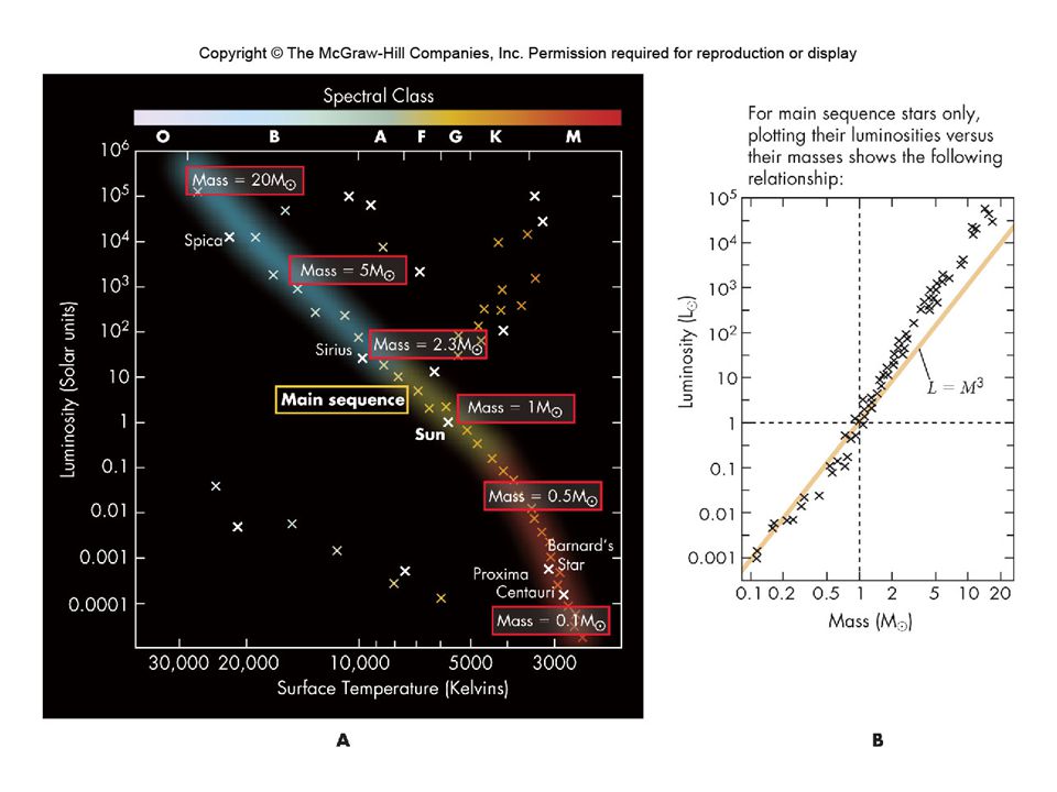
53. The HR Diagram
The H-R diagram is a plot of stellar temperature vs luminosity
Interestingly, most of the stars on the H-R diagram lie along a smooth diagonal running from hot, luminous stars (upper left part of diagram) to cool, dim ones (lower right part of diagram)

54. The HR Diagram
By tradition, bright stars are placed at the top of the H-R diagram and dim ones at the bottom, while high-temperature (blue) stars are on the left with cool (red) stars on the right (Note: temperature does not run in a traditional direction)

55. The HR Diagram
The diagonally running group of stars on the H-R diagram is referred to as the main sequence
Generally, 90% of a group of stars will be on the main sequence; however, a few stars will be cool but very luminous (upper right part of H-R diagram), while others will be hot and dim (lower left part of H-R diagram)

56. Analyzing the HR Diagram
The Stefan-Boltzmann law is a key to understanding the H-R diagram
For stars of a given temperature, the larger the radius, the larger the luminosity
Therefore, as one moves up the H-R diagram, a star’s radius must become bigger
On the other hand, for a given luminosity, the larger the radius, the smaller the temperature
Therefore, as one moves right on the H-R diagram, a star’s radius must increase
The net effect of this is that the smallest stars must be in the lower left corner of the diagram and the largest stars in the upper right

57. Analyzing the HR Diagram

58. Giants and Dwarfs
Stars in the upper left are called red giants (red because of the low temperatures there)
Stars in the lower right are white dwarfs
Three stellar types: main sequence, red giants, and white dwarfs

59. Giants and Dwarfs
Giants, dwarfs, and main sequence stars also differ in average density, not just diameter
Typical density of main-sequence star is 1 g/cm3, while for a giant it is 10-6 g/cm3

60. The Mass-Luminosity Relation
Main-sequence stars obey a mass-luminosity relation, approximately given by:
L and M are measured in solar units
Consequence: Stars at top of main-sequence are more massive than stars lower down

61. Luminosity Classes
Another method was discovered to measure the luminosity of a star (other than using a star’s apparent magnitude and the inverse square law)
It was noticed that some stars had very narrow absorption lines compared to other stars of the same temperature
It was also noticed that luminous stars had narrower lines than less luminous stars
Width of absorption line depends on density: wide for high density, narrow for low density

62. Luminosity Classes

63. Luminosity Classes
Luminous stars (in upper right of H-R diagram) tend to be less dense, hence narrow absorption lines
H-R diagram broken into luminosity classes: Ia (bright supergiant), Ib (supergiants), II (bright giants), III (giants), IV (subgiants), V (main sequence)
Star classification example: The Sun is G2V

65. Summary of the HR Diagram
Most stars lie on the main sequence
Of these, the hottest stars are blue and more luminous, while the coolest stars are red and dim
Star’s position on sequence determines its mass, being more near the top of the sequence
Three classes of stars:
Main-sequence
Giants
White dwarfs

66. Variable Stars
Not all stars have a constant luminosity – some change brightness: variable stars
There are several varieties of stars that vary and are important distance indicators
Especially important are the pulsating variables – stars with rhythmically swelling and shrinking radii

67. Mira and Cepheid Variables
Variable stars are classified by the shape and period of their light curves – Mira and Cepheid variables are two examples

68. The Instability Strip
Most variable stars plotted on H-R diagram lie in the narrow “instability strip”

69. Polaris is a classic Population I Cepheid variable (although it was once thought to be Population II due to its high galactic latitude). Since Cepheids are an important standard candle for determining distance, Polaris (as the closest such star) is heavily studied. Around 1900, the star luminosity varied ±8% from its average (0.15 magnitudes in total) with a 3.97 day period; however the stars heat is a at a low level. Over the same period, the star has brightened by 15% (on average), and the period has lengthened by about 8 seconds each year.
Recent research reprted in Science suggests that Polaris is 2.5 times brighter today than when Ptolemy observed it (now 2mag, antiquity 3mag). Astronomer Edward Guinan considers this to be a remarkable rate of change and is on record as saying that "If they are real, these changes are 100 times larger than [those] predicted by current theories of stellar evolution.

70. Method of Standard Candles
Step 1: Measure a star’s brightness (B) with a photometer
Step 2: Determine star’s Luminosity, L
Use combined formula to calculate d, the distance to the star
Sometimes easier to use ratios of distances
Write Inverse-Square Law for each star
Take the ratio:

71. Summary

72. Problem 17 Chapter 13
Since t Ceti and a Centauri B have nearly the same luminosity, they are both the same kind of “standard candle” and the difference in apparent magnitudes is a brightness difference that results from one being farther away than the other. The difference in apparent magnitude for the two stars is 2.16, so the ratio of brightness is =7.3. This means a Centauri B appears 7.3 times brighter than t Ceti, it must be closer. Using the method of standard candles from section 13.8,
Bnear /Bfar = (dfar/dnear)2 so 7.3 = (dfar/dnear)2
2.7 = dfar/dnear
This means t Ceti is 2.7 times farther away than a Centauri B.

73. M = (L)(1/3) = (5000)(1/3) = 17 solar masses.
Problem 15
From the chapter, L ≈ M3 when the values are in solar units. If L = 5000,
M = (L)(1/3) = (5000)(1/3) = 17 solar masses.
Problem 13, Two Stars in a Binary System.
In this problem we want to know the separation between the stars. We again use the modified form of Kepler’s Third Law,
m + M = a3/P2.
m+M is 8 solar masses, and P is 1 year,
8 = a3/ 12
a3 = 8 × 1
a = 81/3 = 2 AU.
The separation in the binary is 2AU.

74. Problem 10. A line in a star’s spectrum is 402
Problem 10. A line in a star’s spectrum is nanometers in the laboratory. The same line lies at nanometers in a star’s spectrum. How fast is the star moving along the line of sight? Is it moving toward or away from us.
The wavelength we measure, l, is shorter than the “rest” wavelength, lo, measured in the lab. The object is blueshifted, which means that it is approaching us.
l = 400 nm l o = nm
Dl = l - lo = –0.2 nm
Using the Doppler shift formula, V = (Dl/lo ) × c, where V = object’s velocity, and
c = speed of light = 3 × 105 km/s,
V = (–0.2 nm / nm) × 3 × 105 = –150 km/s
The velocity comes out negative because the star is approaching us (l - lo< 0).

75. Problem 8. A stellar companion of Sirius has a temperature of 27,000 K and a Luminosity of 1/100 L (sun). What is its radius compared to the Earth’s.
For the white dwarf companion of Sirius, called Sirius B:
T = 27,000 K, L = 10-2Lo
L = 4pR2 s T4 so R = (L/4ps T4)1/2
The radius goes as L1/2 times T4/2= T2, so compared to the Sun’s radius, if Sirius B has 1/100 the luminosity and a temperature 27,000K/6,000 K = 4.5 times as much as the Suns,
R = (1/100) 1/2 (4.5) -2 Ro = 1/10 × 1/20.25 Ro = Ro
The white dwarf star, Sirius B, is only about the radius of the Sun. The Earth is about 1/100 = 0.01 as wide as the Sun, so Sirius B is about half the radius of the Earth.