1. Can we image melt with seismic surface waves? Don Forsyth, with very extensive help from Yingjie Yang, Rob Dunn and Dayanthie Weeraratne 1.Powerful new techniques for imaging regional structure with surface waves 2.Good attenuation measurements are essential 3.Very low shear velocities in regions of melt production require relaxed moduli without high attenuation in the seismic frequency band

2. Temperature dependent attenuation and elasticity provide a satisfactory quantitative explanation of the low-velocity zone except in the immediate vicinity of the ridge. Stixrude and Lithgow-Bertelloni, JGR, 2005 The low velocity zone, commonly observed below ocean basins, and its tendency to become less pronounced and deeper with increasing lithospheric age, can be explained by solid state mechanisms without the presence of melt or fluids. Faul and Jackson, EPSL, 2005. The seismic low velocity zone beneath the Pacific results simply from the effect of temperature. The observed decrease in V s as the melting point is approached is due to temperature alone and not due to the presence of melt. Priestley and McKenzie, EPSL, 2006. Is Melt Imaged in the Mantle?

3. Short period Love waves propagating along the East Pacific Rise (Dunn and Forsyth, JGR, 2003?)

7. Very low shear velocities in region of melt production beneath the East Pacific Rise (Dunn and Forsyth, 2003)

8. Finite frequency response kernels for Rayleigh waves (Zhou et al., 2004)

9. Propagate Rayleigh waves from all azimuths through random velocity field with imbedded checkerboard. Seismometers only within checkerboard region. (Yang and Forsyth, GJI, 2006) km

10. Relative amplitudes within checkerboard region for initially plane Rayleigh wave propagating from north. Period is 50 s. Example of amplitude variations in MELT array for event propagating from Kuriles. Represent incoming wavefield as sum of two plane waves. Focusing effects from heterogeneities within and near array represented by response kernels. (Forsyth and Li, 2005)

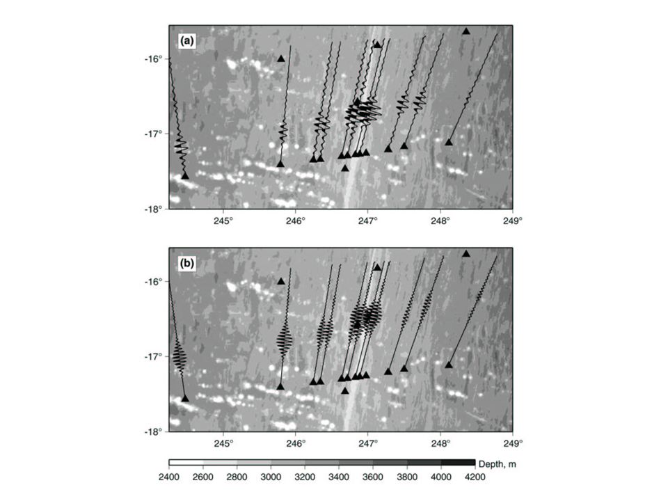
11. Top, inversion for phase velocity with no external heterogeneities. Triangles indicate station locations. Bottom, inversion with random external heterogeneities.

12. Yang and Forsyth, JGR, in press

13. We use well-distributed sources to perform surface wave tomography within S. California. Average phase velocities as a function of period are inverted to give a reference model of shear velocity versus depth. There is a high velocity lid or lithosphere overlying a pronounced low velocity zone.

15. At each period from 25 s to ~145 s we determine the lateral variations in phase velocities using finite frequency sensitivity kernels for both amplitude and phase. A sampling of some of the periods shows gradual evolution in pattern from one period to the next. Longer periods penetrate deeper into the earth. Note very low velocities beneath eastern edge of the Sierra Nevada at short periods. Resolution degrades somewhat towards edges of maps, but 1% variation is significant at ~ 95% confidence level.

16. A slice near the base of the lithosphere shows pattern of both upwellings and downwellings. The low velocity anomaly beneath the Sierra Nevada and Walker Lane (SNWLA) indicates delamination of the mantle part of the lithosphere. GVA is Great Valley anomaly, sometimes called Central Valley anomaly or Isabella anomaly, which has been described as a lithospheric drip. ETRA and WTRA are Eastern and Western Transverse Range anomalies. STA is Salton Trough anomaly.

17. At 70 to 90 km, low velocity region coincides with region of Quaternary volcanism (black dots). Dashed line indicates extent of high-K volcanism at ~ 3.5 Ma. Solid line indicates total extent of volcanism at that time (after Manley et al., Geology, 2000). Note more circular shape of the Great Valley anomaly.

18. Great Valley drip merges with high velocity anomaly beneath eastern Sierra Nevada at 110-130 km depth and is absent deeper than 130 km. Delaminated lithosphere beneath the Sierras seems to have sunk vertically. Transverse Range anomaly clearly separates into two separate drips. Western one dips to the north. Although perhaps initiated by shortening across San Andreas bend, the pattern of anomalies does not appear to be kinematically driven by surface plate motions. The Peninsular Range may have undergone delamination similar to that in the Sierra Nevada. At 70-90 km, low velocities beneath eastern PR merges with Salton Trough anomaly. High velocity anomaly begins at ~130 km and strengthens downward.

19. Great Valley drip may be connected to delaminated lithosphere beneath Sierra Nevada and Owens Valley. Very low velocities at shallow depths indicate partial melt. Transverse Range anomalies separate into two separate drips that extend no deeper than 150 km. Peninsular Range delamination does not extend to as shallow depths as beneath Sierra Nevada and top of delaminated lithosphere is deeper.

20. Priestly and McKenzie, EPSL, 2006 Empirical fit to variation of Vs with age. “The activated process responsible for the rapid decrease in Vs as the melting point is approached is presumably the same as that responsible for the corresponding decrease in Q.”

21. Faul and Jackson, EPSL, 2005

22. Typically, background, temperature-dependent Q -1 is assumed to be of form Q -1 ( ,T) = A [  exp(H/RT)] -   where  ~.2 to.3 For Q -1 << 1, V  T) = V 0 (T)[1 - cot  2) Q -1 ( ,T)/2] V 0 may be a function of T, P, and melt concentration. Plus, there may be band-limited absorption mechanisms in the presence of melt. Melt squirt,through which pressure differences between inclusions are equalized by melt transport,is expected to operate outside the seismic frequency band (Hammond and Humphreys, JGR, 2000). Elastically accommodated grain boundary sliding in the presence of melt may produce a broad absorption peak in the seismic band (Faul et al., JGR, 2004)

23. Jackson et al, JGR, 2004

24. Hammond and Humphreys, JGR, 2000 Faul et al., JGR, 2004

25. Faul and Jackson, EPSL,2005

26. Yang, Weeraratne, Forsyth, in prep

27. Solve for attenuation and velocity simultaneously using two plane waves to represent distant effects on wavefield, response kernels to represent regional effects, station corrections to represent local response, and correct for spherical spreading of wave. Left shows residual amplitudes (event amplitudes normalized to 1.0) as a function of distance from closest station for GLIMPSE at 25 s when attenuation is neglected. Right shows attenuation coefficient  f/UQ. Amplitude A = A o exp(-  x). GLIMPSE MELT

29. Conclusions Powerful new imaging techniques find very low shear velocities in melt producing regions in the mantle, but Q values are not as low as expected. Shear velocities may be affected by attenuation and relaxation of the elastic moduli outside the seismic frequency band. Melt squirt could be responsible, requiring 0.5 - 1.0% melt using realistic melt geometries (Hammond and Humphreys, 2000). Beneath old seafloor, the presence of water may be responsible for lowering S velocity and increasing attenuation in the asthenosphere, rather than temperature alone.