Download presentation
Presentation is loading. Please wait.

1
Computing Classic Closeness Centrality, at Scale Edith Cohen Joint with: Thomas Pajor, Daniel Delling, Renato Werneck Microsoft Research

2
Very Large Graphs Model many types of relations and interactions (edges) between entities (nodes) Call detail, email exchanges, Web links, Social Networks (friend, follow, like), Commercial transactions,… Need for scalable analytics: Centralities/Influence (power/importance/coverage of a node or a set of nodes): ranking, viral marketing,… Similarities/Communities (how tightly related are 2 or more nodes): Recommendations, Advertising, Prediction
 between entities (nodes) Call detail, exchanges, Web links, Social Networks (friend, follow, like), Commercial transactions,… Need for scalable analytics: Centralities/Influence (power/importance/coverage of a node or a set of nodes): ranking, viral marketing,… Similarities/Communities (how tightly related are 2 or more nodes): Recommendations, Advertising, Prediction")
3
Centrality Centrality of a node measures its importance. Applications: ranking, scoring, characterize network properties. Several structural centrality definitions: Betweeness: effectiveness in connecting pairs of nodes Degree: Activity level Eigenvalue: Reputation Closeness: Ability to reach/influence others.

4
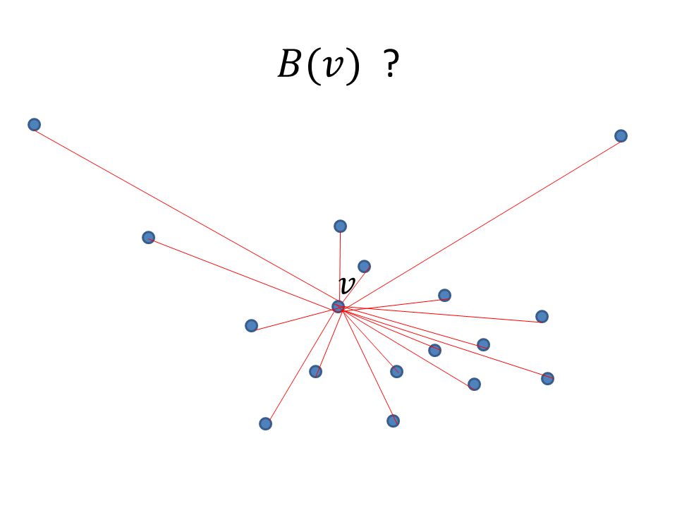
Closeness Centrality Classic Closeness Centrality [(Bavelas 1950, Beaucahmp 1965, Sabidussi 1966)] (Inverse of) the average distance to all other nodes Maximum centrality node is the 1-median Importance measure of a node that is a function of the distances from a node to all other nodes.
![Closeness Centrality Classic Closeness Centrality [(Bavelas 1950, Beaucahmp 1965, Sabidussi 1966)] (Inverse of) the average distance to all other nodes Maximum centrality node is the 1-median Importance measure of a node that is a function of the distances from a node to all other nodes.](http://images.slideplayer.com/13/3842749/slides/slide_4.jpg "Closeness Centrality Classic Closeness Centrality [(Bavelas 1950, Beaucahmp 1965, Sabidussi 1966)] (Inverse of) the average distance to all other nodes Maximum centrality node is the 1-median Importance measure of a node that is a function of the distances from a node to all other nodes.")
5
Computing Closeness Centrality

6
Exact, but does not scale for many nodes on large graphs.

7
Goals

8
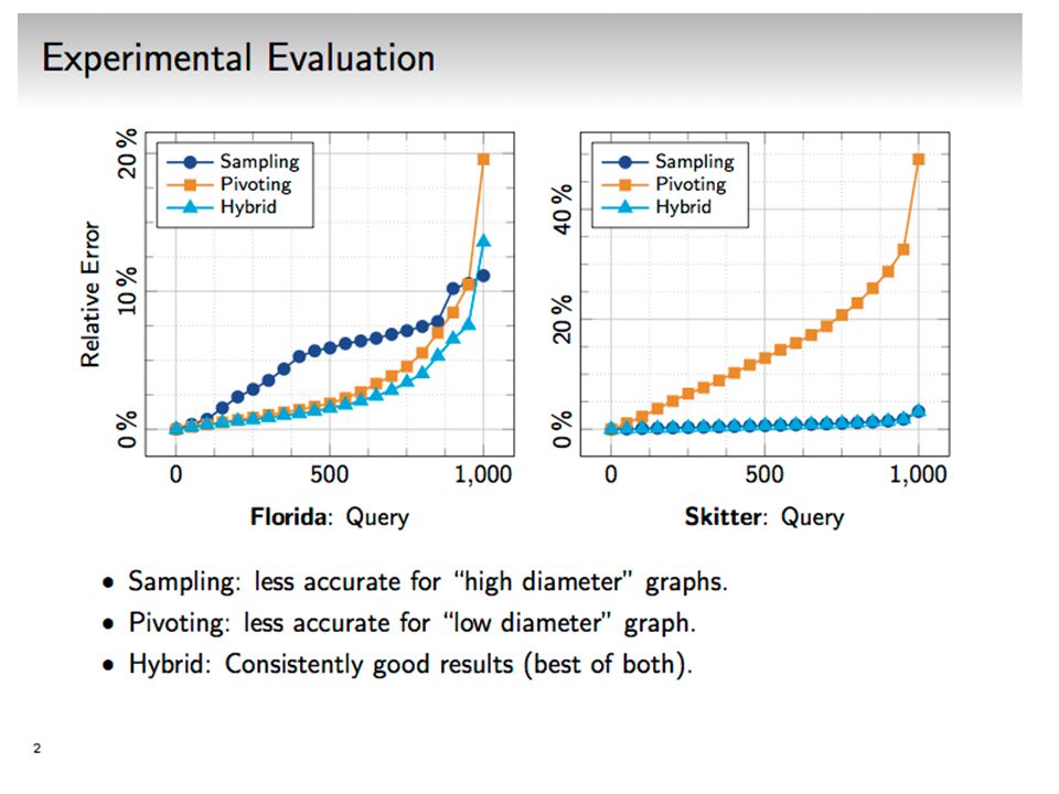
Algorithmic Overview Approach I: Sampling Properties: good for “close” distances (concentrated around mean) Approach II: Pivoting Properties: good for “far” distances (heavy tail) Hybrid: Best of all worlds
 Approach II: Pivoting Properties: good for far distances (heavy tail) Hybrid: Best of all worlds")
9
Approach I: Sampling [EW 2001, OCL2008,Indyk1999,Thorup2001] Computation Estimation
![Approach I: Sampling [EW 2001, OCL2008,Indyk1999,Thorup2001] Computation Estimation](http://images.slideplayer.com/13/3842749/slides/slide_9.jpg "Approach I: Sampling [EW 2001, OCL2008,Indyk1999,Thorup2001] Computation Estimation")
10
Sampling

13
Sampling: Properties Works well! sample average captures population average

14
Sampling: Properties Heavy tail -- sample average has high variance

15
Approach II: Pivoting Computation Estimation

16
Pivoting

19
Inherit centrality of pivot (closest sampled node)
")
20
Pivoting: properties

21
WHP

22
Pivoting: properties Bounded relative error for any instance ! A property we could not obtain with sampling

23
Pivoting vs. Sampling But neither gives us a small relative error !

24
Hybrid Estimator !! How to partition close/far ?

25
Hybrid

26
Close nodes Far nodes

27
Close nodes

28
Far nodes

29
Analysis

30
Analysis (worst case)
")
31
Analysis What about the guarantees (want confidence intervals) ?
")
32
Adaptive Error Estimation Idea: We use the information we have on the actual distance distribution to obtain tighter confidence bounds for our estimate than the worst-case bounds. Close nodes: Estimate population variance from samples.

33
Extension: Adaptive Error Minimization For a given sample size (computation investment), and a given node, we can consider many thresholds for partitioning into closer/far nodes. We can compute an adaptive error estimate for each threshold (based on what we know on distribution). Use the estimate with smallest estimated error.
. Use the estimate with smallest estimated error..")
34
Efficiency

35
Scalability: Using +O(1)/node memory
/node memory")
36
Hybrid slightly slower, but more accurate than sampling or pivoting

41
Directed graphs Sampling works (same properties) when graph is strongly connected. Pivoting breaks, even with strong connectivity. Hybrid therefore also breaks. When graph is not strongly connected, basic sampling also breaks – we may not have enough samples from each reachability set (Classic Closeness) Centrality is defined as (inverse of) average distance to reachable (outbound distances) or reaching (inbound distances) nodes only. We design a new sampling algorithm…
 Centrality is defined as (inverse of) average distance to reachable (outbound distances) or reaching (inbound distances) nodes only. We design a new sampling algorithm….")
42
…Directed graphs (Classic Closeness) Centrality is defined as (inverse of) average distance to reachable (outbound distances) or reaching (inbound distances) nodes only. Process nodes u in random permutation order Run Dijkstra from u, prune at nodes already visited k times

43
Directed graphs: Reachability sketch based sampling is orders of magnitude faster with only a small error.

44
Extension: Metric Spaces Perform both a forward and back Dijkstra from each sampled node. Compute roundtrip distances, sort them, and apply estimator to that. Application: Centrality with respect to Round-trip distances in directed strongly connected graphs:

45
Extension: Node weights Weighted centrality: Nodes are heterogeneous. Some are more important. Or more related to a topic. Weighted centrality emphasizes more important nodes. Variant of Hybrid with same strong guarantees uses a weighted (VAROPT) instead of a uniform nodes sample.
 instead of a uniform nodes sample..")
46
Closeness Centrality Classic (penalize for far nodes) Distance-decay (reward for close nodes) Different techniques required: All-Distances Sketches [C’ 94] work for approximating distance-decay but not classic.
![Closeness Centrality Classic (penalize for far nodes) Distance-decay (reward for close nodes) Different techniques required: All-Distances Sketches [C’ 94] work for approximating distance-decay but not classic.](http://images.slideplayer.com/13/3842749/slides/slide_46.jpg "Closeness Centrality Classic (penalize for far nodes) Distance-decay (reward for close nodes) Different techniques required: All-Distances Sketches [C’ 94] work for approximating distance-decay but not classic.")
47
Summary

48
Thank you!

Similar presentations


 edge (u,v) denotes similarity between u and v weighted.>")


