1. Aerosol, Interhemispheric Gradient, and Climate Sensitivity Ching-Yee Chang Department of Geography University of California Berkeley Lawrence Livermore National Lab Seminar April 27, 2011 Collaborators: John Chiang (UC Berkeley) Michael Wehner (Lawrence Berkeley Lab)

2. Sulfate Aerosols and Climate Difference in SAT caused by sulfate aerosol indirect effect (Rotstayn & Lohmann 2002) Direct forcing from anthropogenic sulfate forcing (Kiehl & Briegleb 1993) IPCC AR4

3. Large uncertainty in the aerosol forcing Kiehl 2007 IPCC AR4

4. Outline Sulfate aerosol control of Tropical Atlantic climate over the 20 th century (Chang et al. 2011, in press for Journal of Climate) Projection of the Interhemispheric Gradient in 21 st century Interhemispheric Gradient and Transient Climate Response

5. Sulfate aerosol control of Tropical Atlantic climate over the 20 th century

6. Atlantic interhemispheric SST gradient over the 20 th century Interhemispheric SST index = South – North box 21-yr running mean on annual mean data Hadley SST, ERSST, Kaplan SST HADISST ERSST KAPLAN SST

7. Ensemble Empirical Mode Decomposition (EEMD) Modes from Ensemble Empirical Mode Decomposition (EEMD) analysis: Multidecadal (mode 4) and trend (mode 5) HADISST ERSST KAPLAN SST

8. The interhemispheric SST gradient and the meridional position of ITCZ Mode 1 of an MCA of SSTA and 10m winds, and regression of the SSTA mode 1 time series on precipitation (Chiang and Vimont, 2004)

9. Equatorial meridional winds ICOADS Winds Smith et al. 2010: Reconstructed global precip CRU TS 2.1 land precip. south-north June-July-August precipitation

10. CMIP3 models simulation of Atlantic Interhemispheric Gradient in 20 th century climate experiment

11. Variance explained by this EOF: 49% Most of the projection coefficient are positive (Most models have a upward trend in the SSTA gradient indices) Projection of EOF1 onto each run 1 st EOF of AITG indices from 71 model runs South Hemisphere warming more than North Hemisphere This trend mitigates after 1980

12. T-test value=4.41 p-value = 0.00001 (assuming 71 d.o.f. for the 20 th century runs, and 44 for the preindustrial) Mean of 1900-1982 trend in SSTA gradient significantly different from preindustrial run Unit: 0.1K/100yr

13. Regression of SSTA onto model-index EOF1 Hadley SSTA Stronger warming in the South Atlantic Model ensemble averaged SSTA

14. Southward shift of ITCZ Regression of Precip. Anomaly onto model-index EOF1 Model ensemble averaged Precip. anomaly CRU Precip. anomaly

15. Attribution the cause of the trend  Trend behavior appears in model ensemble mean  Most likely to be externally forced  Single forcing runs

16. Results from single forcing runs CCSM3 (2 members) PCM1 (4 members) GISS modelE (1 member)s ) SST gradient index ITCZ index most resembles the 1st EOF of the indices of the 20C expt.

17. CCSM3 sulfate aerosol emission forcing data CCSM3 simulated sulfate aerosol optical depth

18. EOF1 from different subsets of models  EOF1 from AIE models capture the turn of the trend better  AIE models simulate the AITG trend closer to observation AIE models: Models with both Aerosol Direct and Indirect Effect No-AIE models: Models with only aerosol direct, but no Indirect Effect X-axis unit: 0.1K/100yr

19. Modeled SSTA and Precip.A regression on model-index EOF1 Warming asymmetry and ITCZ southward shift stronger in AIE models Models with Aerosol Indirect Effect Models without Aerosol Indirect Effect

20. Summary I  Interhemispheric gradient of Atlantic SST found to have an upward trend before 1980, indicating stronger warming in the South Atlantic and southward shift of ITCZ  A similar positive trend is detected in the IPCC models.  This trend is likely due the north-south disparity in anthropogenic sulfate aerosol emissions

21. 3 different scenarios are examined A1B, A2, B1 Both Atlantic and Pacific sectors Projection of the Interhemispheric Gradient in 21 st century Indices are defined as south box minus north box

22. Global mean of various anthropogenic forcing agents in future scenarios IPCC AR4 WG1, Fig.10.26

23. 95-year (2004~2098) trend statistics Pacific Atlantic A1B A2 B1 Most models project downward trend of the Pacific index in the 21th century in these 3 future scenarios => North Pacific warming stronger than South Less conclusive results on the projection of the Atlantic index trend X-axis unit: 0.1K/100yr

24. A1B Atmos. Sulfate burden unit: 10e-6 kg/m2 Pacific Atlantic High-lat index (35~60) Tropical index (5~35) Stronger change in the interhemispheric gradient of sulfate aerosol forcing across the equator in the Pacific sector (From miub_echo model) It’s projected that most of the decrease of sulfate aerosol mainly comes from Asia More aerosol emission from Tropical Atlantic than from North Atlantic

25. Atmospheric Sulfate burden A1bA2 B1 All three scenarios have stronger change in sulfate aerosol forcing across the equator in the Pacific sector

26. 1%/yr to 2xCO 2 experiment However, similar change of Pacific gradient is found in 1%/yr to double CO2 experiment, but with weaker magnitudes

27. Comparison: 1%/yr to 2xCO2 and A1B experiments (Yr60~Yr80) – ( Yr1~Yr20 )(2079~2098) – ( 2005~2024 )

28.  Most models project negative trend in the Pacific interhemispheric gradient – the rate of the warming in the north Pacific speeds up at the end of 21 st century  Possibly related to the decrease of the aerosols in the north Pacific in the future, but GHG forcing or other factors may also contribute Summary II

29. Interhemispheric Gradient and Climate sensitivity

30. Trend Statistic from different subsets of models  AIE models simulate the AITG trend closer to observation AIE models: Models with both Aerosol Direct and Indirect Effect No-AIE models: Models with only aerosol direct, but no Indirect Effect X-axis unit: 0.1K/100yr

31. Kiehl 2007: Total forcing inversely correlated to climate sensitivity Large uncertainty in the aerosol forcing

32. Equilibrium Climate sensitivity and Transient Climate Response Equilibrium Climate Sensitivity IPCC AR4 Table 8.2 Transient Climate Response 300 ppm 600 ppm CO2 concentration + Slab ocean AGCM T0 T’ CO2 concentration AGCM + OGCM 300 ppm 600 ppm T0 T’

33. Climate sensitivity and Transient Climate Response IPCC AR4 Table 8.2

34. Atlantic SSTA Grad. Trend v.s. Climate Sensitivity There seems to be a linear relationship between the gradient trend and the Transient Climate Response (TCR) among most of the models

36. Regional Transient Climate response Regional Transient Climate Responses (TCR) in the Tropical Atlantic regions are similar in the North and South Roughly a linear relationship between regional TCR and global TCR

37. A linear relationship between TCR and Interhemispheric Gradient Trend Similar regional TCRs, in the Tropical Atlantic region across the equator Roughly a linear relationship between regional TCR and global TCR Models with higher TCR are models with stronger aerosol forcing, due to the constraint of the 20C global mean SAT change Stronger aerosol forcing with larger TCR => stronger SST gradient If we also constrain the models with observed interhemispheric gradient change?

38. Summary III A linear relationship between the modeled Atlantic SST Interhemispheric Gradient and Transient Climate Response for most of the models This relationship can be explained by the uncertainty of the aerosol forcings among the models Further confirms that the important role of aerosol on the change of the Interhemispheric Gradient Constraint on the simulation of Interhemispheric Gradient change (or trend) may be a way to confine the uncertainty of models’ climate sensitivity

39. Thank you for your attention

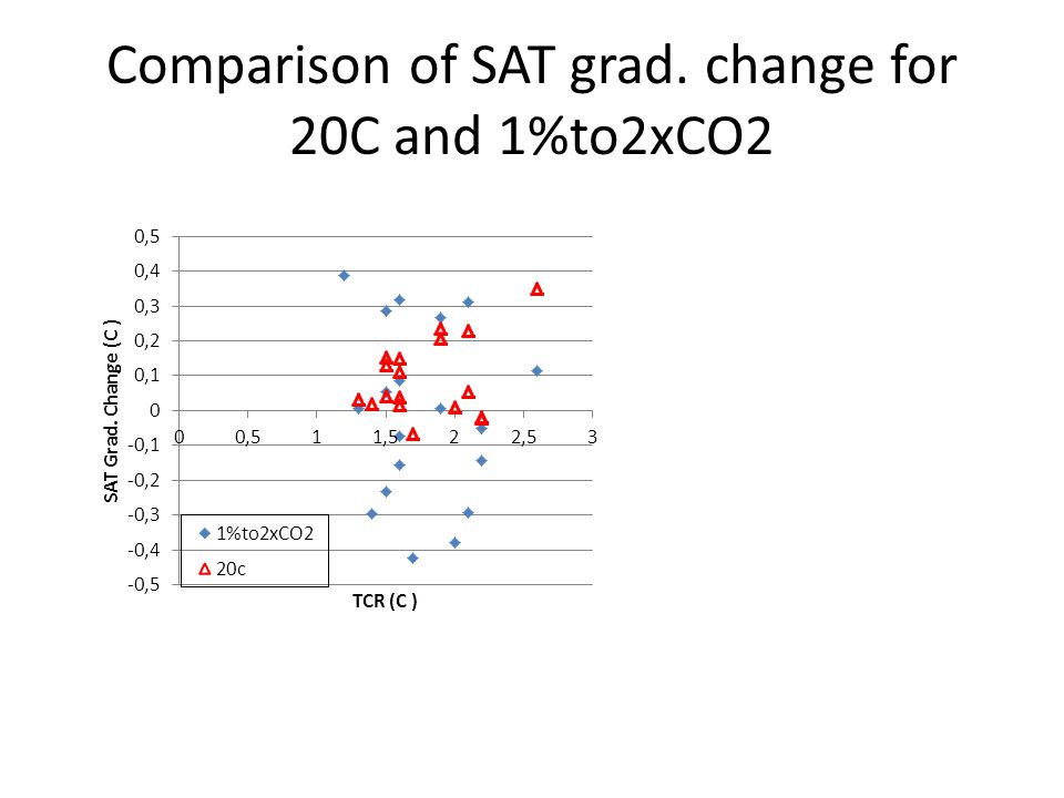
40. Comparison of SAT grad. change for 20C and 1%to2xCO2

42. Climate sensitivity and total anthropogenic forcing In general, 20 Century temperature change = climate sensitivity × Radiative Forcing Smaller total anthropogenic forcing, larger climate sensitivity Larger total anthropogenic forcing, smaller climate sensitivity Let Consistent with Kiehl 2007

43. Regional TCR and interhemispheric gradient South – North Gradient change, △ G Linear relationship btw. TCR and interhemispheric gradient change

44. Model internal averaged Gradient change

46. Pacific and Atlantic Interhemispheric Gradient HADISST ERSST(NOAA) KAPLAN SST Pacific Atlantic

47. 20C experiment PacificAtlantic 49% 51% EOF1 from all models Projection of EOF1 on each run

48. A1B B1 A2 Atlantic Interhemispheric SST Gradient

49. Pacific Interhemispheric SST Gradient A1B B1 A2