1. Meso-NH model 40 users laboratories http://www.aero.obs-mip.fr/mesonh A research model, jointly developped by Meteo-France and Laboratoire d’Aérologie (CNRS/UPS)

2. Plan IntroductionIntroduction Clouds : MCS, Cyclones, Cu, Sc, FogClouds : MCS, Cyclones, Cu, Sc, Fog Dynamics of Boundary layers : Stable, ConvectiveDynamics of Boundary layers : Stable, Convective Chemistry, Dusts, ElectricityChemistry, Dusts, Electricity Coupling : C02, Hydrology, DispersionCoupling : C02, Hydrology, Dispersion Applications : Duct mapping, climatologyApplications : Duct mapping, climatology AROMEAROME

3. Types of simulations A broad range of resolution from synoptic scales (  x~10km), meso-scale (  x~1km) to Large Eddy Simulation (  x~10m) Real cases (from ECMWF, ARPEGE, ALADIN analyses or forecasts)Real cases (from ECMWF, ARPEGE, ALADIN analyses or forecasts) Ideal cases  unrealistic casesIdeal cases  unrealistic cases - Academic cases (validation of the dynamics) - Basic studies (Diurnal cycle …) : Cloud Resolving Model (CRM) - To reproduce an observed reality (via forcings) (intercomparison : GCSS, EUROCS …) Simulations 3D, 2D, 1D

4. Lafore Moncrieff 89 Stratiform Density Current Convective H D A tropical squall line (P.Jabouille) : Idealized simulation according to a real case (COPT81) U W 

5. Cloud dropletsRain drops Pristine iceGraupel Snow Jabouille. Caniaux et al., 1994

6. (Keil et Cardinali, 2003) 32km : 150x150 8km : 145x145 2km : 150x150 over 51 levels IOP8 (F<1) IOP2a (F>1) 8 km 2 km Monte Lema S Pol Ronsard ECMWF  32 km 3 Doppler radars ( ) Orographic precipitation 3D (MAP) How can dynamics modify the microphysics ? Lascaux et Richard, 2005

7. Snow Graupel Hail Cloud Rain Ice IOP2a IOP2a ( Strong convection) - Deep system (unblocked unstable case, high Fr) - Large amount of hail and graupel - Main process : Riming Mean vertical distribution of hydrometeors IOP8 ( Stratiform event) - Shallow system (blocked case, low Fr) -Large amount of snow - Main process : Vapor deposition on snow IOP8 Snow Lascaux et Richard, 2005 Orographic precipitation 3D (MAP)

8. Impact de la convection sur la stationnarité d’un système Ctrl Noc 4h-accumulated rainfall 18-22 UTC on 8 Sept. 2002 Noc = without evaparative cooling Ctrl = with evaporative cooling Nuissier et Ducrocq, 2006 Strong convective events on SE of FRANCE How can mycrophysics modify the dynamics ? Cev. ‘95 Gard ‘02 Aude ‘99 1D-  budget over the MCS (convective + stratiform).

9. max : 135 mm max : 25 mm m mm Quasi-stationnary MCS 13-14 Oct. 1995 Cumulated precipitation 01 UTC to 06 UTC the 14 th Oct. 1995 MESO-NH,  x=10km max: 31 mm MESO-NH,  x=2.5kmOBSERVATIONS (Ducrocq et al, 2002) Initial conditions: ARPEGE analysis at 18UTC m MESO-NH,  x=2.5km Initialisation Ducrocq et al (2000)’s max : 99 mm

10. Impact de la pollution sur le cycle diurne du stratocumulus 0.7g/kg 700m r c (g/kg) Simulation LES 50m Nuage non pollué Sandu, I., 2007 0TU 61218243036 Impact d’une atmosphère polluée sur le cycle diurne = Effet indirect des aérosols L’évaporation liée à la bruine empêche la stratification à la base du nuage et le découplage LWP (g/m²)

11. FOG – 1D simulation – Temporal evolution on 18h from 18TU rc Without cloud droplet sedimentation With cloud droplet sedimentation With cloud droplet sedimentation but a coarser vertical resolution Rémi, S., 2006

12. Simulation of cyclone : case of Dina 7800 km,  x=36km 1944 km,  x=12km 720 km,  x=4km 3600 km Automatic method of Initialization : Filtering/Bogussing Barbary et al.

13. Vertical cross-sections at  x=4km K m/s K Horizontal wind S-N W-E Barbary et al.

14. Plan IntroductionIntroduction Clouds : MCS, Cyclones, Cu, Sc, FogClouds : MCS, Cyclones, Cu, Sc, Fog Dynamics of Boundary layers : Stable, ConvectiveDynamics of Boundary layers : Stable, Convective Chemistry, Dusts, ElectricityChemistry, Dusts, Electricity Coupling : C02, Hydrology, DispersionCoupling : C02, Hydrology, Dispersion Applications : Duct mapping, climatologyApplications : Duct mapping, climatology AROMEAROME

15. Couche limite stable : application à l’île de Majorque 2 1 Motivation : Comment les flux nocturnes s’organisent en l’absence de gradient synoptique fort ? Cuxart et al.  x=1km  z=3m dans les 200 premiers m 4TU SE N 50 km * * 55 km NE Forte stratification des vents à l’aéroport Direction du vent Force du vent

16. Influence des effets locaux : la brise de mer Urban network Model Lemonsu et al., 2005a Température de l’air 26 June 2001, 1400 UTC 26 Juin 2001 : Marseille sous l’influence d’écoulements locaux, induisant des mécanismes complexes au dessus de la ville

17. Influence des effets locaux : la brise de mer VAL OBS CNRS Puget Massif Marseille veyre City centre z = 400 m AGL VAL OBS CNRS m s -1 Puget Massif Marseille veyre City centre z = 50 m AGL West SSB South SSB South- East DSB Horizontal wind field 26 June 2001, 1400 UTC Lemonsu et al., 2005a

18. 6 m s -1 420-2-4-6 26 June 2001, 1400 UTC B C D A TWL B C D A Model VDOL City center 02460246 Distance (km) VDOL City center 0.5 1.0 1.5 2.0 2.5 Altitude (km) 500 400 300 200 100 50 ZS (m) Marseillev eyre 190 o Puget Massif CNRS (Radar) 3 km VAL (Lidar) OBS (Radar) Etoile Massif Comparison with transportable wind lidar (TWL) Lemonsu et al., 2005a

19. Couche limite convective : variabilité de la vapeur d’eau Vols avions P3Vols avions KA Histogramme de w à Z=0.4z i.... max _ _ min Histogramme de  à Z=0.4z i Histogramme de rv à Z=0.4z i Enveloppe max. Enveloppe min. Modèle Lidar 8km 1500m Descentes d’air sec Thermiques Couvreux, F., 2005

20. Plan IntroductionIntroduction Clouds : MCS, Cyclones, Cu, Sc, FogClouds : MCS, Cyclones, Cu, Sc, Fog Dynamics of Boundary layers : Stable, ConvectiveDynamics of Boundary layers : Stable, Convective Chemistry, Dusts, ElectricityChemistry, Dusts, Electricity Coupling : C02, Hydrology, DispersionCoupling : C02, Hydrology, Dispersion Applications : Duct mapping, climatologyApplications : Duct mapping, climatology AROMEAROME

21. OZONE le 25 Juin 2001 9 UTC 9km 3km <30ppb Parc Naturel VerdonMarseille 85ppb MarseilleParc Naturel Verdon >90ppb 15 UTC >90ppb Cousin et Tulet, 2004

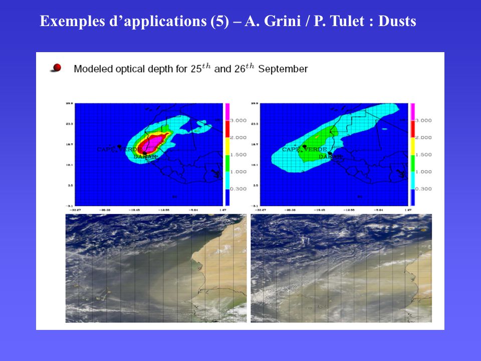
22. surface Infiltration d’eau Réservoir profond Réservoir superficiel Sol Nu ou Rochers Lessivage aérosols Absorption/ diffusion Du rayonnement solaire Refroidissement surface Aérosols Désertiques – Génération – Transport - Effets u* turbulence Émission Saltation Exemples d’applications (5) – A. Grini / P. Tulet : Dusts

24. Barthe et al. [2005] + + - Explicite electrical scheme in Meso-NH Local separation of charges Transfert and transport of charges Microphysical and dynamical processes Electric field Lightning parameterization Bidirectional leader (determinist) Vertical extension of the lightning Channel steps (probabiliste) Horizontal extension of the lightning Charge neutralization E > E trig yes no

25. Life cycle of electrical charges in a convective cell Barthe et Pinty, JGR Apparition of graupel Electrization of the cloud Apparition of electric field lightning Triggering of convection Simulation Méso-NH

26. Plan IntroductionIntroduction Clouds : MCS, Cyclones, Cu, Sc, FogClouds : MCS, Cyclones, Cu, Sc, Fog Dynamics of Boundary layers : Stable, ConvectiveDynamics of Boundary layers : Stable, Convective Chemistry, Dusts, ElectricityChemistry, Dusts, Electricity Coupling : C02, Hydrology, DispersionCoupling : C02, Hydrology, Dispersion Applications : Duct mapping, climatologyApplications : Duct mapping, climatology AROMEAROME

27. Atmospheric CO 2 modelling : the Meso-NH model Online coupling with the surface scheme ISBA-A-gs :   CO 2 surface fluxes : - assimilation (<0) CO2 absorption by vegetation - respiration (>0) CO2 emissions from ecosyst. depends on temperature - anthropogenic emissions (>0) and ocean fluxes (<0 in our latitude)   Feedback : CO 2 concentrations variations from the atmosphere to the surface ISBA-A-g s Meteorological Model LE, H, Rn, W, Ts… Atmospheric [CO 2 ] concentrations Anthropogenic Sea Meso-NH Surface Lafore et al., 98 Noilhan et al. 89, 96, Calvet et al., 98 CO 2 Fluxes

28. Atmospheric CO 2 modelling : May – 27 2005 Boundary layer heterogeneity Sarrat et al., 2006 Concentration CO2 (ppm)

29. Atmospheric CO 2 modelling May – 27 2005 : comparisons obs/simu Simulated vertical cross section of CO 2 Ocean - Marmande Agricultural area Forest area Vertical cross section of observed CO 2 by aircraftoceanforestcropland forestcropland Sarrat et al., 2006 Winter crops  Assimilation Forêt  Respiration

30. Vidourle Gard Cèze Ardèche TOPMODEL (Beven and Kirkby, 1979) distributed hydrologic model with one model by basin : 9 basins (200-2200 km²) Objectives : - Flow and rapide flood forecasts - Retroaction of the hydrology on the atmosphere - Available for AROME HYDROLOGY : Development of the coupling Meso-NH-ISBA-TOPMODEL K.Chancibault et al., CNRM/GMME/MICADO

31. SPRAY Lagrangian particle model At least 10000 particles released Advection+Turbulence+random Applied to the 2 Meso-NH grids  PERLE P E R L E  PERLE (Programme d’Evaluation des Rejets Locaux d’Effluents) Dispersion Meso-NH 2 grids (Regional  x=8km, L=240km/ Local  x=2km, L=60km) 36 levels until 16km ALADIN initialization and coupling Meso-scale meteorology Will be exported to AROME Modelling system for environmental emergency

33. Plan IntroductionIntroduction Clouds : MCS, Cyclones, Cu, Sc, FogClouds : MCS, Cyclones, Cu, Sc, Fog Dynamics of Boundary layers : Stable, ConvectiveDynamics of Boundary layers : Stable, Convective Chemistry, Dusts, ElectricityChemistry, Dusts, Electricity Coupling : C02, Hydrology, DispersionCoupling : C02, Hydrology, Dispersion Applications : Duct mapping, climatologyApplications : Duct mapping, climatology AROMEAROME

34. Roses Aladin 3 ansMéso-NH 95 datesMeasurements North Alps

35. Applications : Détermination de conduits de propagation d’ondes électromagnétiques. Pourret, V., 2006 : PEA PREDEM Co-indice de réfraction N=(77.6/T).(P+4810.e/T)-6.e/T Sommet du conduit de propagation = Altitude de l’inversion de M co-indice de réfraction OG dans le sillage des îles au sommet du conduit Réfraction normale Réfraction vers le bas

36. AROME : Application of Researh to Operations at MEsoscale Future non-hydrostatic model 2.5km resolution Dynamics based on ALADIN-NH (semi-implicite, semi- lagrangian) Data assimilation ALADIN 3D-VAR Physics based on Méso-NH : microphysics ICE3, Turbulence 1D, shallow convection, externalised surface

37. Arome 60s Case of Gard, initial bogus Lame d’eau 12-22 Tu radar de Nîmes > 300 mm Couplage : Aladin 3h Forecasts MésoNH 4s 304 mm 274 mm MésoNH –  t= 4s, CPU = 24h20 AROME –  t =60s, CPU = 2h30