Download presentation
Presentation is loading. Please wait.

1
Image Blending and Compositing 15-463: Computational Photography Alexei Efros, CMU, Fall 2010 © NASA

2
Image Compositing

3
Compositing Procedure 1. Extract Sprites (e.g using Intelligent Scissors in Photoshop) Composite by David Dewey 2. Blend them into the composite (in the right order)
 Composite by David Dewey 2. Blend them into the composite (in the right order).")
4
Need blending

5
Alpha Blending / Feathering 0 1 0 1 + = I blend = I left + (1- )I right
I right")
6
Affect of Window Size 0 1 left right 0 1

7
Affect of Window Size 0 1 0 1

8
Good Window Size 0 1 “Optimal” Window: smooth but not ghosted

9
What is the Optimal Window? To avoid seams window = size of largest prominent feature To avoid ghosting window <= 2*size of smallest prominent feature Natural to cast this in the Fourier domain largest frequency <= 2*size of smallest frequency image frequency content should occupy one “octave” (power of two) FFT
 FFT.")
10
What if the Frequency Spread is Wide Idea (Burt and Adelson) Compute F left = FFT(I left ), F right = FFT(I right ) Decompose Fourier image into octaves (bands) –F left = F left 1 + F left 2 + … Feather corresponding octaves F left i with F right i –Can compute inverse FFT and feather in spatial domain Sum feathered octave images in frequency domain Better implemented in spatial domain FFT
 Compute F left = FFT(I left ), F right = FFT(I right ) Decompose Fourier image into octaves (bands) –F left = F left 1 + F left 2 + … Feather corresponding octaves F left i with F right i –Can compute inverse FFT and feather in spatial domain Sum feathered octave images in frequency domain Better implemented in spatial domain FFT")
11
Octaves in the Spatial Domain Bandpass Images Lowpass Images

12
Pyramid Blending 0 1 0 1 0 1 Left pyramidRight pyramidblend

13
Pyramid Blending

14
laplacian level 4 laplacian level 2 laplacian level 0 left pyramidright pyramidblended pyramid

15
Laplacian Pyramid: Blending General Approach: 1.Build Laplacian pyramids LA and LB from images A and B 2.Build a Gaussian pyramid GR from selected region R 3.Form a combined pyramid LS from LA and LB using nodes of GR as weights: LS(i,j) = GR(I,j,)*LA(I,j) + (1-GR(I,j))*LB(I,j) 4.Collapse the LS pyramid to get the final blended image
 = GR(I,j,)*LA(I,j) + (1-GR(I,j))*LB(I,j) 4.Collapse the LS pyramid to get the final blended image")
16
Blending Regions

17
Horror Photo © david dmartin (Boston College)
")
18
Results from this class (fall 2005) © Chris Cameron
 © Chris Cameron")
19
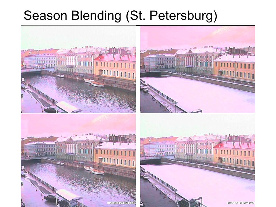
Season Blending (St. Petersburg)
")
21
Simplification: Two-band Blending Brown & Lowe, 2003 Only use two bands: high freq. and low freq. Blends low freq. smoothly Blend high freq. with no smoothing: use binary alpha

22
Low frequency ( > 2 pixels) High frequency ( < 2 pixels) 2-band Blending
 High frequency ( < 2 pixels) 2-band Blending")
23
Linear Blending

24
2-band Blending

25
Don’t blend, CUT! So far we only tried to blend between two images. What about finding an optimal seam? Moving objects become ghosts

26
Davis, 1998 Segment the mosaic Single source image per segment Avoid artifacts along boundries –Dijkstra’s algorithm

27
min. error boundary Minimal error boundary overlapping blocksvertical boundary _ = 2 overlap error

28
Seam Carving http://www.youtube.com/watch?v=6NcIJXTlugc

29
Graphcuts What if we want similar “cut-where-things- agree” idea, but for closed regions? Dynamic programming can’t handle loops

30
Graph cuts – a more general solution n-links s t a cut hard constraint hard constraint Minimum cost cut can be computed in polynomial time (max-flow/min-cut algorithms)
")
31
Kwatra et al, 2003 Actually, for this example, DP will work just as well…

32
Lazy Snapping Interactive segmentation using graphcuts

33
Gradient Domain In Pyramid Blending, we decomposed our image into 2 nd derivatives (Laplacian) and a low-res image Let us now look at 1 st derivatives (gradients): No need for low-res image –captures everything (up to a constant) Idea: –Differentiate –Blend / edit / whatever –Reintegrate
 and a low-res image Let us now look at 1 st derivatives (gradients): No need for low-res image –captures everything (up to a constant) Idea: –Differentiate –Blend / edit / whatever –Reintegrate")
34
Gradient Domain blending (1D) Two signals Regular blending Blending derivatives bright dark
 Two signals Regular blending Blending derivatives bright dark")
35
Gradient Domain Blending (2D) Trickier in 2D: Take partial derivatives dx and dy (the gradient field) Fidle around with them (smooth, blend, feather, etc) Reintegrate –But now integral(dx) might not equal integral(dy) Find the most agreeable solution –Equivalent to solving Poisson equation –Can be done using least-squares
 Trickier in 2D: Take partial derivatives dx and dy (the gradient field) Fidle around with them (smooth, blend, feather, etc) Reintegrate –But now integral(dx) might not equal integral(dy) Find the most agreeable solution –Equivalent to solving Poisson equation –Can be done using least-squares")
36
Perez et al., 2003

37
Perez et al, 2003 Limitations: Can’t do contrast reversal (gray on black -> gray on white) Colored backgrounds “bleed through” Images need to be very well aligned editing
 Colored backgrounds bleed through Images need to be very well aligned editing")
38
Gradients vs. Pixels Can we use this for range compression?

39
Thinking in Gradient Domain Our very own Jim McCann:: James McCann Real-Time Gradient-Domain Painting, SIGGRAPH 2009

40
Gradient Domain as Image Representation See GradientShop paper as good example: http://www.gradientshop.com/

41
Can be used to exert high-level control over images

42
gradients – low level image-features

43
Can be used to exert high-level control over images gradients – low level image-features +100 pixel gradient

44
Can be used to exert high-level control over images gradients – low level image-features gradients – give rise to high level image-features +100 pixel gradient

45
Can be used to exert high-level control over images gradients – low level image-features gradients – give rise to high level image-features +100 pixel gradient +100 pixel gradient

46
Can be used to exert high-level control over images gradients – low level image-features gradients – give rise to high level image-features +100 pixel gradient +100 pixel gradient image edge

47
Can be used to exert high-level control over images gradients – low level image-features gradients – give rise to high level image-features manipulate local gradients to manipulate global image interpretation +100 pixel gradient +100 pixel gradient

48
Can be used to exert high-level control over images gradients – low level image-features gradients – give rise to high level image-features manipulate local gradients to manipulate global image interpretation +255 pixel gradient

49
Can be used to exert high-level control over images gradients – low level image-features gradients – give rise to high level image-features manipulate local gradients to manipulate global image interpretation +255 pixel gradient

50
Can be used to exert high-level control over images gradients – low level image-features gradients – give rise to high level image-features manipulate local gradients to manipulate global image interpretation +0 pixel gradient

51
Can be used to exert high-level control over images gradients – low level image-features gradients – give rise to high level image-features manipulate local gradients to manipulate global image interpretation +0 pixel gradient

52
Can be used to exert high-level control over images gradients – give rise to high level image-features

53
Can be used to exert high-level control over images gradients – give rise to high level image-features Edges

54
Can be used to exert high-level control over images gradients – give rise to high level image-features Edges object boundaries depth discontinuities shadows …

55
Can be used to exert high-level control over images gradients – give rise to high level image-features Edges Texture

56
Can be used to exert high-level control over images gradients – give rise to high level image-features Edges Texture visual richness surface properties

57
Can be used to exert high-level control over images gradients – give rise to high level image-features Edges Texture Shading

58
Can be used to exert high-level control over images gradients – give rise to high level image-features Edges Texture Shading lighting

59
Can be used to exert high-level control over images gradients – give rise to high level image-features Edges Texture Shading lighting shape sculpting the face using shading (makeup)
")
60
Can be used to exert high-level control over images gradients – give rise to high level image-features Edges Texture Shading lighting shape sculpting the face using shading (makeup)
")
61
Can be used to exert high-level control over images gradients – give rise to high level image-features Edges Texture Shading lighting shape sculpting the face using shading (makeup)
")
62
Can be used to exert high-level control over images gradients – give rise to high level image-features Edges Texture Shading lighting shape sculpting the face using shading (makeup)
")
63
Can be used to exert high-level control over images gradients – give rise to high level image-features Edges Texture Shading

64
Can be used to exert high-level control over images gradients – give rise to high level image-features Edges Texture Shading Artifacts

65
Can be used to exert high-level control over images gradients – give rise to high level image-features Edges Texture Shading Artifacts noise sensor noise

66
Can be used to exert high-level control over images gradients – give rise to high level image-features Edges Texture Shading Artifacts noise seams seams in composite images

67
Can be used to exert high-level control over images gradients – give rise to high level image-features Edges Texture Shading Artifacts noise seams compression artifacts blocking in compressed images

68
Can be used to exert high-level control over images gradients – give rise to high level image-features Edges Texture Shading Artifacts noise seams compression artifacts ringing in compressed images

69
Can be used to exert high-level control over images gradients – give rise to high level image-features Edges Texture Shading Artifacts noise seams compression artifacts flicker flicker from exposure changes & film degradation

70
Can be used to exert high-level control over images

71
Optimization framework Pravin Bhat et al

72
Optimization framework Input unfiltered image – u

73
Optimization framework Input unfiltered image – u Output filtered image – f

74
Optimization framework Input unfiltered image – u Output filtered image – f Specify desired pixel-differences – ( g x, g y ) min ( f x – g x ) 2 + ( f y – g y ) 2 f Energy function
 min ( f x – g x ) 2 + ( f y – g y ) 2 f Energy function")
75
Optimization framework Input unfiltered image – u Output filtered image – f Specify desired pixel-differences – ( g x, g y ) Specify desired pixel-values – d min ( f x – g x ) 2 + ( f y – g y ) 2 + ( f – d ) 2 f Energy function
 Specify desired pixel-values – d min ( f x – g x ) 2 + ( f y – g y ) 2 + ( f – d ) 2 f Energy function")
76
Optimization framework Input unfiltered image – u Output filtered image – f Specify desired pixel-differences – ( g x, g y ) Specify desired pixel-values – d Specify constraints weights – ( w x, w y, w d ) min w x ( f x – g x ) 2 + w y ( f y – g y ) 2 + w d ( f – d ) 2 f Energy function
 Specify desired pixel-values – d Specify constraints weights – ( w x, w y, w d ) min w x ( f x – g x ) 2 + w y ( f y – g y ) 2 + w d ( f – d ) 2 f Energy function")
80
Least Squares Example Say we have a set of data points (X1,X1’), (X2,X2’), (X3,X3’), etc. (e.g. person’s height vs. weight) We want a nice compact formula (a line) to predict X’s from Xs: Xa + b = X’ We want to find a and b How many (X,X’) pairs do we need? What if the data is noisy? Ax=B overconstrained
 We want a nice compact formula (a line) to predict X’s from Xs: Xa + b = X’ We want to find a and b How many (X,X’) pairs do we need. What if the data is noisy. Ax=B overconstrained.")
81
Putting it all together Compositing images Have a clever blending function –Feathering –Center-weighted –blend different frequencies differently –Gradient based blending Choose the right pixels from each image –Dynamic programming – optimal seams –Graph-cuts Now, let’s put it all together: Interactive Digital Photomontage, 2004 (video)
")
Similar presentations


>")


 Segmentation Carsten Rother Vladimir Kolmogorov Andrew Blake Antonio Criminisi Geoffrey Cross [based on Siggraph.>")


 – camera parameters for.>")


 Main topic: Feature detection.>")
 go quickly...>")


