1. Niches and Areas of Distribution I Jorge Soberon Museum of Natural History, University of Kansas Photo by Warren Apel

2. Caveat Emptor This is a talk about ideas being developed as we speak. Nothing is yet firmly established We encourage dissent and questioning Key papers: –Pulliam, 2000, Ecol. Lett. 3:349-361 –Pearson & Dawson, 2003, Glob. Ecol. Biogeog. 12:361-371 –Araujo & Guisan, 2005, Glob. Ecol. Biogeog. 33:1677-1688 –Kearny 2006, Oikos 115: 186-191 –Soberon & Peterson, 2005, Biodiv. Info. 2:1-10 –Soberon 2007, Ecol. Lett. 10:1115-1123

3. Purpose: to clarify very muddled terminology We need concepts of “area of distribution” of a species which are clear and operational. The same for niche. Relate the concepts of “areas of distribution” and “niche”.

4. Around 1990 three things happened 1.Large databases of presences of species (mainly computerized scientific collections) began being accessible at significant amounts

5. II. GIS… Geographical Information Systems technology became widely accessible to ecologists and biogeographers

6. III. “Niche” Modeling Since the 1980s, the Australians began doing “bioclimatic” modeling for applied entomology purposes (Climex) Later they developed Bioclim, DOMAIN, and then, GARP Today, there are about 15 methods to do niche modeling, most of them in freeware form

7. Using those tools… Since about 1995 there has been an explosion in the application of ecological “niche” modeling methods to estimate “areas of distribution”, potential or actual. The methods are used to predict invasive-species routes, spread of vectors of diseases, restoration ecology, conservation, and many topics in fundamental ecology and biogeography. Literally hundreds of papers have been published, about the potential and/or actual distributions of thousands of species

8. And yet… “Geographic distributional areas are the shadows produced by taxa on the geographical screen. To study them one needs to measure ghosts” –A. Rapoport. Areography: Geographical Strategies of Species, 1982 “Most ecologists would agree that niche is a central concept of ecology, even though we do not know exactly what it means” –L. Real and S. Levin, Theoretical advances: the role of theory in the rise of modern ecology 1991

9. In other words: We (the niche modelers) are doing wholesale estimation of those shadows (geographical areas) by using a non- concept (niche)! Not nice…

10. We need to define ENM terms and methodology Preferably operational definitions Relevant in the field of modeling distribution areas Preferably mathematical (formal) Avoid breaking with tradition, if possible

11. Let us begin with area. In books they appear as little maps Some theorists even treat them as if they were physical entities. But areas are composed by the presence (detected) of individuals Jim Brown suggested a Gedankenexperiment

12. Imagine that we make individuals fluoresce...

14. We see that to define “area of distribution” we need to: Agree on what it is meant by a “presence” (sink or source populations). Potential or actual. Agree at what resolutions makes sense to talk about areas of distribution? Normally, this would be “low resolutions” > 10 3 km 2 Inside the cells, we are in the domain of ecology, outside, it is biogeography or macroecology

15. So areas are... Regions of the world defined by the detection of individuals within cells in grids There are several things that we can detect: reproductive individuals, just individuals, regions with positive growth rates... Although a lot of those can be defined at high resolutions, areas are defined at low resolutions. It is still a dream to measure the movements of all the individuals of a species...

16. What determines where do we find individuals? Autoecology, interactions, migration patterns, historical factors, operating with different strenghts at different spatiotemporal scales. There are equations (horribly difficult) describing this. Species Grid cell

17. Grinnell, scenopoetic Elton, bionomic Movements G BAM Diagram B M A

18. So we can define stuff… We can define, rigorously, areas of distributions in terms of whether the x i j (t) are positive, or above a threshold, or whether the intrinsic growth rate is positive (potential area of distribution)

19. And niches? Clearly, the spatial regions determined by the parameters in those horrible equations have environments. Niches may be defined using the environmental variables in the “occupied” cells.

20. A useful and forgotten distinction of Hutchinson (1978) Scenopoetic variables. Non-interacting, slowly changing from a species point of view. Bionomic variables. Coupled, fast changing Hutchinson´s nice distinction was quickly forgotten and then reinvented by Austin, Begon, and others.

21. Niches can be defined using the same equations that govern area Fundamental niche Intrinsic Growth Rate (Scenopoetic) Resource-consumer dynamics, competitors, predator-prey (bionomic). Migration colonization, history

22. So, the niches are the sets of environments present in the different areas: An abiotic niche: the set of environments in the area where the intrinsic growth rate is positive A colonizable niche: the set of environments in the area where both biotic and abiotic conditions are right A occupied niche, the set of the environments in the area where the species actually occurs

23. Hutchinson´s terminology 1.Fundamental niche. Defined without reference to scenopetic and biotic variables. 2.Realized niche. Fundamental reduced by competition. The entire biotope occupied 1.Abiotic niche. Defined using only scenopoetic variables. 2.Colonizable niche. The abiotic reduced by competition. 3.Occupied niche. The realized niche taking into account movement restrictions

24. Some areas and niches B M JOJO J´ O B M JOJO A Occupied = colonizable? AbioticColonizable and occupied

25. The Eltonian Noise Hypothesis I. At the scale at what we work (cells > 10 0 km 2 ), the biotic factors become much less relevant than the abiotic ones: the signal is dominated by abiotic factors, and the biotic factors act as noise B M JOJO A J´ O

26. Eltonian noise hypothesis II. The Eltonian processes are of very high resolution In the large cells at which scenopoetic variables are measured “competitive exclusion” may take place without affecting the totality of populations. A B M

27. Examples and counterexamples Cactoblastis cactorum Obligate pollinators

28. Extremely Important I. By assuming non-interactivity we can represent the environments (and therefore the Grinnell niches) by sets of numbers. The interactive and dynamic Elton niches must be represented by the parameters of functions (sometimes by the isoclines), because one needs to measure both the use of a resource and its impact (see Chase and Leibold, 2003, Ecological Niches)

29. Extremely Important II. Since we are defining our Grinnell niches using such “scenopoetic” variables, it means that we can use: –Widely available datasets –At low resolutions

30. Towards concluding… So it is useful to define areas as subsets of cells in a geographic grid, defined by biological properties of species (presence, presence of viable populations, suitable conditions for survivorship,…) And Grinnell niches as the subsets of scenopoetic variables associated to those areas

31. And of course, Grinnell niches are multidimensional, but in the space of scenopoetic variables “The concept of niche...is here defined as the sum of all the environmental factors acting on an organism; the niche thus defined is a region of an n- dimensional hyperspace”

32. Multidimensionality applies to both scales of niches In Grinnell´s (related to distribution, geographic), variables are elevation, orientation, geology, climate... These variables are “less interactive” In Elton´s (more trophic, ecological), variables may be nutrient concentrations, food size distributions, prey, predators, competitors and mutualist densities... These variables are highly interactive

33. So, it is useful to accept tow levels Grinnell Niches, low resolution, scenopoetic variables. Elton Niches, high resolution, bionomic variables. They may be the cause of reduction from Fundamental to Realized A M B

34. This distinction is based on: Accepting the assumption that differences in certain extreme types of variables: non-interactive, meaningful at low resolutions, vs interactive, meaningful at high resolutions do exist. How valid is this simplification? The fact that ENM is predictive is evidence in favor. We need to establish the scope of validity of the assumption. At high resolutions probably it will break down.

35. Thanks to Town Peterson, Richard Pearson, Enrique Martinez, Miguel Nakamura, Carlos Martinez del Rio, the students of the Niche Seminar

36. Niches and Areas of Distribution II Jorge Soberon Museum of Natural History, University of Kansas Photo by Warren Apel

37. So how we measure a Grinnell Niche? 1.We go and see where it is that a species occurs (“…without immigration”) 2.We measure environmental variables in those places. 3.We extrapolate from a few “points” to an area. 4.We obtain the corresponding environmental values. 5.This is the niche.

38. There are Several Ways of Calculating the Niche Physical variable 1 Physical variable 2 Bioclim Clusters About 15 others...

39. G-space. Two dimensions Low resolution (pixels of 1 km 2 ) E-space. Many variables. Scenopoetic. Low resolution. Low precision

40. Notice: Conceptually, every algorithm tries to “recover” the realized Grinnell niche, since the data points come from the actual distribution J O 1.However, when we map back from E to G, in general, we do not recover J O since there may be other spatial regions with the same niche. We recover J C. In general, one has to deal with this problem outside the niche modeling algorithm JOJO NONO J´ O

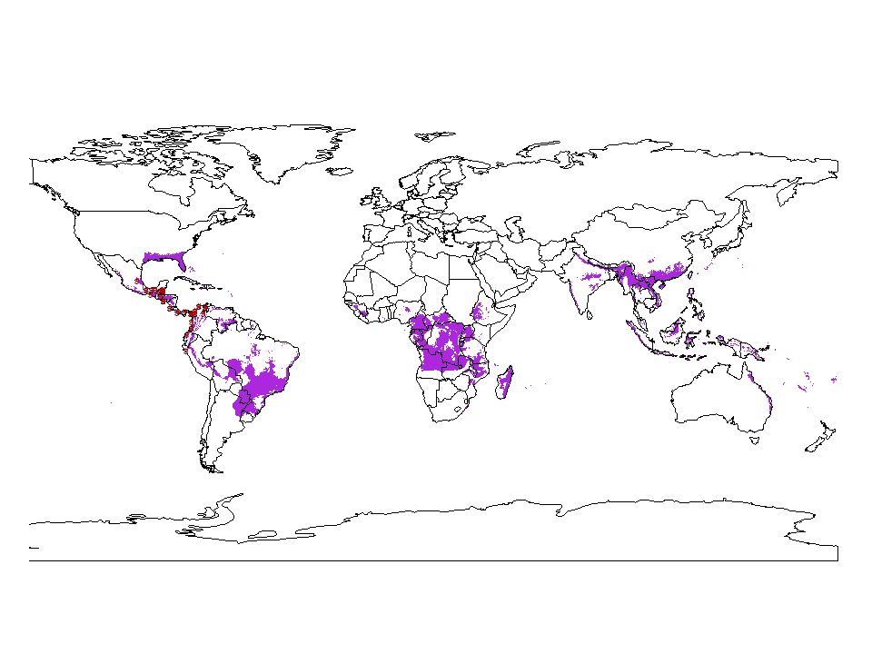
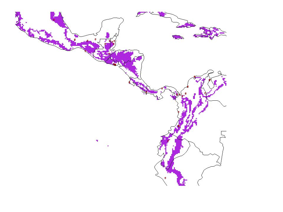
41. Tamandua mexicana

43. When  -1 (N O ) is different from J O ? J1J1 J2J2 E1E1 G-space E-space

44. Using Garp, Maxent, GAM, … estimate the Occupied Niche If you want the Jo (rather than J C ), then clip the geographical extent of the E R using biological connectivity or historical reasoning. With GIS display the geographical extent of the Occupied Niche Begin with presence (absence) data

45. A real-life example: Baronia brevicornis and its single food plant, Acacia cochliacantha

46. For this example the following layers were used, all at 1:1,000,000: Aspect Elevation Mean Temperature Average minimum daily temperature Average maximum daily temperature Yearly precipitation MME about 500 meters

47. B. brevicornis Abiotic Niche using BS Garp

48. II: Estimating the “Area of Accesibility” From where? What is the initial condition? At what scale? In relation to what vagility parameters? At certain scales, one can assume that biogeography is a good surrogate for the accesibility areas, this is, we assume that if a species is present in a given biogeographical region, it can reach all of it.

49. B. brevicornis Biogeographical Provinces

50. B. brevicornis. Biogeographical Provinces as Surrogates for Accesibility Areas

51. B. Brevicornis Niche ∩ Accesibility ∩

52. III. Estimating an Obligate Interaction B. brevicornis only food plant is the legume Acacia cochliacantha A similar analysis is the repeated for A. cochliacantha

53. A. cochliacantha Abiotic Niche

54. A. cochliacantha accesibility region (biogeography)

55. A. cochliacantha niche ∩ accesibility

56. B. brevicornis (red) ∩ A. cochliacantha (blue)

58. Finally, is it the occupied or the abiotic niche? B M JOJO A B M JOJO A

59. Conclusion. We still have a lot to learn, for example about: The process of “reduction” from Abiotic to Occupied, by Eltonian factors. This is a problem in scaling The basic assumption of using ENM to study invasions is that N O = N C. Is this true? When? A more standardized procedure to obtain different Areas and Grinnellian Niches using ENM Developing validation techniques based on different configurations of the BAM diagram And many other things…

60. Acknowledgments Providers of museum data, for the huge effort they have put in collecting, curating and identifying specimens, and then sharing their results The owners of the land where those specimens were originally taken

61. Very Fundamental Concepts: To each region in G-space there are corresponding ones in E-space  (G) = E There is an inverse operation that maps from G to E:   (E) = G E-Space n dimensions G-Space, 2 dimensions

62. More Fundamental Concepts. Niches (Grinnell) are subsets of spaces of environmental variables corresponding to subsets of geographical space where a species live, or can live. The function  that maps from G to E is defined very simply by the tables in the GIS that link coordinates with environmental values. And viceversa, for the relation  -1 that maps back E to G

63. Gedankenexperiment I: We know all regions where intrinsic growth rate is positive (this is, we disregard biotic interactions and movement limitations) G F We agree to call the corresponding Environmental subset the Fundamental Niche, E F =  (G F ) It ought to be true that  -1 (E F )=  -1 (  (G F ))=G F GFGF

64. Gedankenexperiment II: We know now the area of distribution of a species G R We agree to call the corresponding Environmental subset the Realized Niche, E R =  (G R ) Now it is obvious that  -1 (E R ) = may not be = G R GRGR

65. Tamandua mexicana

68. When  -1 (E R ) is different from G R ? G1G1 G2G2 E1E1 G-space E-space