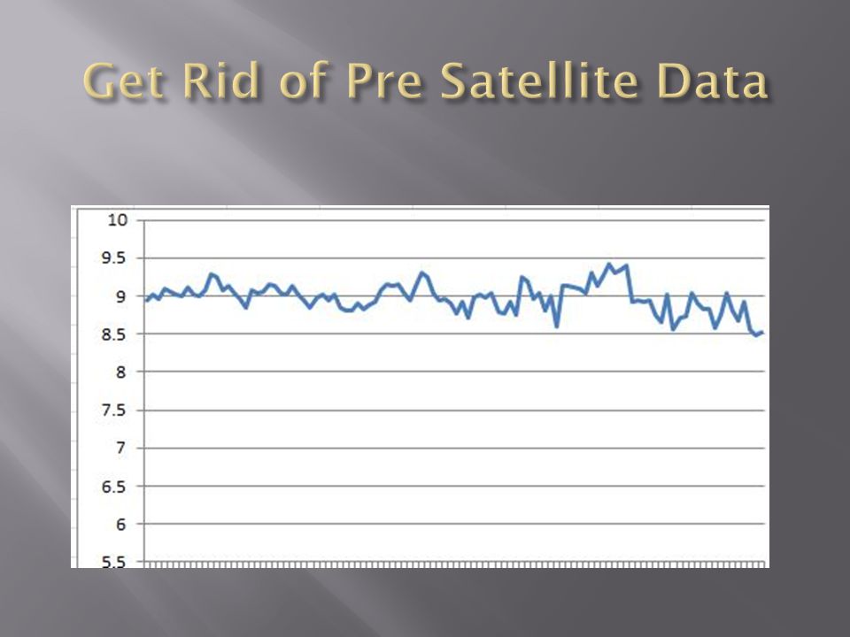
1. All about noisy time series analysis in which features exist and long term behavior is present; finite boundary conditions are always an issue

2.  For any time series problem, plot the data first at some sensible scale and do simple smoothing to see if there is underlying structure vs just all random noise.  Do a simple preliminary VISUAL analysis – fit a line to all or parts of the data, just so you get some better understanding  EXCEL is actually convenient for this

7.  Small differences in approaches produce slightly different results:

9. Area ratio = 1.37 (721/525) No Need to do “fancy” interpolation for numerical integration for this data given the intrinsic noise – why do extra calculations if you don’t need to  spare machine resource

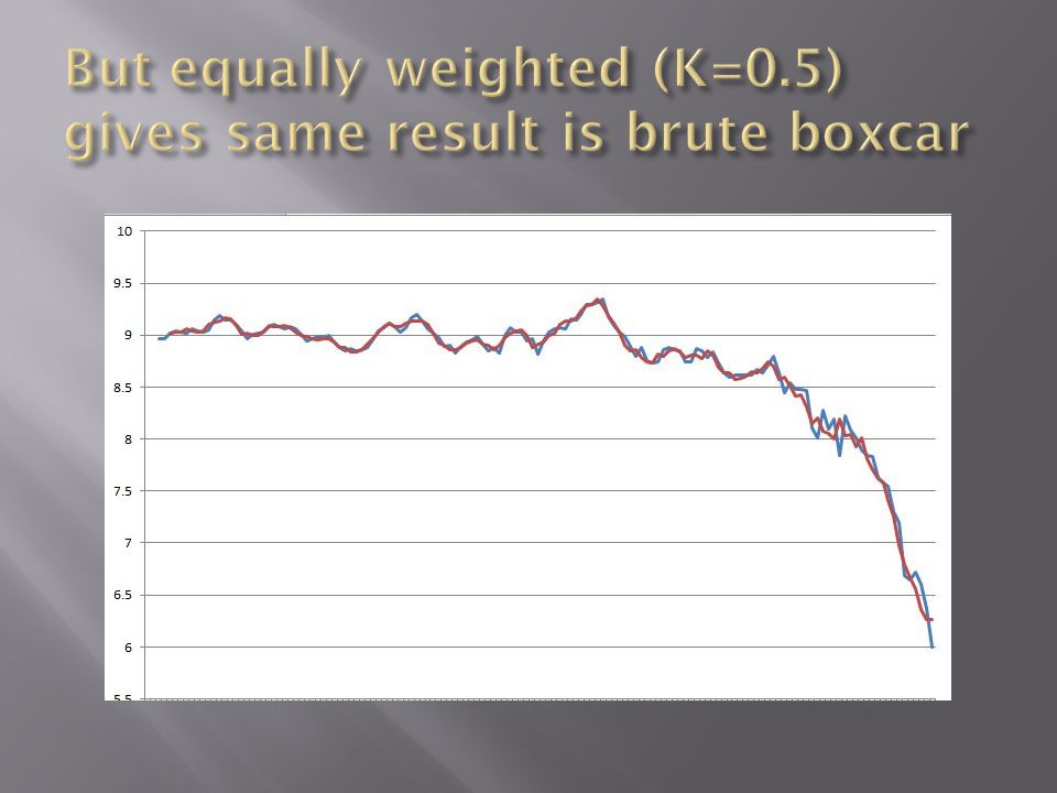
11.  There are many techniques for smoothing  There is always a trade off between smoothing width and data resolution. There is no formula to optimally determine this – you have to experiment with different procedures.  Exponential smoothing often looks “weird” as both the weights and the smoothing changes with smoothing parameter

12. Area under curve = 1 Area under curve = 1; 11 points are shown here; use 7 points for each data point; 96% of wt.

13. Note phase “error” – this is common because of a finite data end so best build in an offset that you can change

18. Blue = exponential

21. Easy and the point was that this is not a randomly distributed variable; distribution is skewed (third moment; kurtosis = 4 th moment

22.  As expected this gave everyone the most trouble; its not hard but you do have to pay attention to the your process.  First produce a sensible plot so you get a feel for the amplitude of the feature

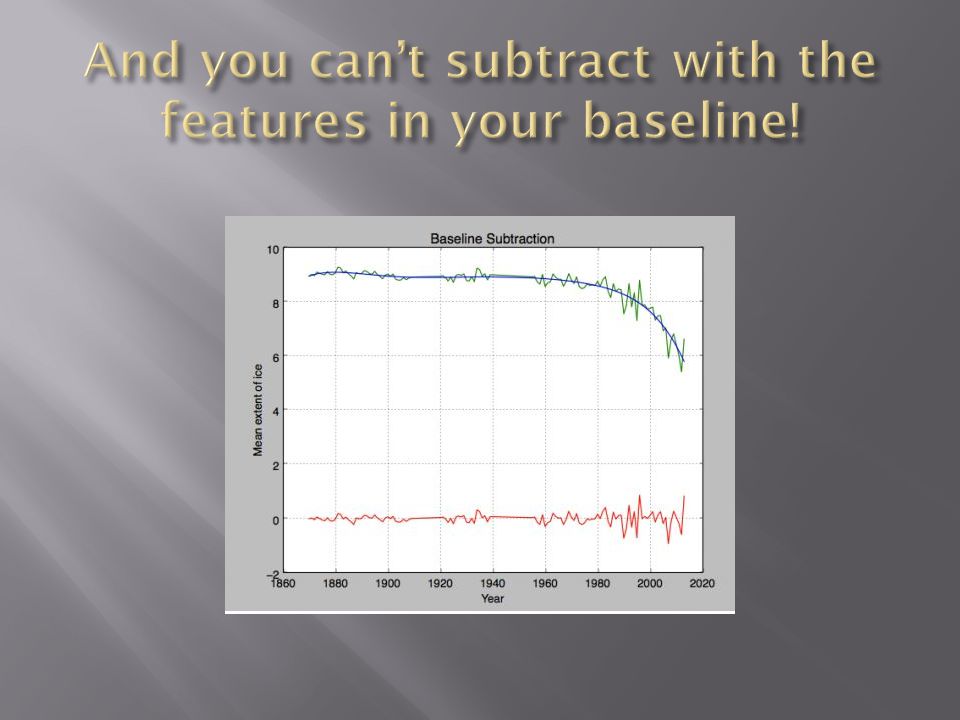
23. See the Noise! Now do Feature Extraction – want to fit a “continuum” that doesn’t include features. This simple linear fit does include features so is wrong but it serves as an initial guide.. What you notice is that the peak is about.4 units above the “baseline”. Window out features and continue. 0.4

31. Maybe 3 events; 1 for sure; note amplitude is correct compared to the first pass (i.e. ~0.4) Area under the curve for biggest feature is about a 3% excess over baseline – not very high amplitude but not a NOISE FEATURE either; 0=9 sq. km; feature is 20 years; 9x20 =180; area of feature is triangle: ½ *20*(.5) = 5; 5/180 = 3% (good enough for estimate) Constant = 9.1

32. >>> import numpy >>> x,y = numpy.loadtxt(“xy.txt”, unpack=True) >>>p = numpy.polyfit(x, y, deg=3) >>>print p >>>-7e-07 1e-04 -0.0072 +9.108 Excel = -5e-07 8e-05 -.0063 9.105

33. Yes there is a family of functions that work for this kind of “sharp cutoff wave form”

34. SIGMOIDAL DISTRIBUTION A = 10.35 B = 17.46 C = 2.2E10 D =-4.69 The zunzun.com site is magic!

35. Science/Policy Issue; 2095 vs 2030