1. Definition and Measurement of Colloids
COAGULATION
Definition and Measurement of Colloids
Many of the contaminants in water and wastewater contain matter in the colloidal form. These colloids result in a stable “suspension”. In general the suspension is stable enough so that gravity forces will not cause precipitation of these colloidal particles. So they need special treatment to remove them from the aqueous phase. This destabilization of colloids is called “coagulation”.

2. Typical colloidal characteristics for water and wastewater:
· Size range: micron. (somewhere in the range between a molecule and bacteria in size).
· 50 – 70 % of the organic matter in domestic wastewater is composed of colloidal matter.
· In water treatment color, turbidity, viruses, bacteria, algae and organic matter are primarily either in the colloidal form or behave as colloids.

3. The following graphic shows some size characteristics for particulates in water and wastewater.

5. Colloidal definition:
Particles which are just big enough to have a surface which is microscopically observable or which is capable of adsorption of another phase.
Size (arbitrary): to 1 micron.
Surface area: ~ 1 sq yd to 1 acre/ gram.

6. For colloids surface properties dominate gravity forces
For colloids surface properties dominate gravity forces. These surface properties prevent the colloids from coming together (coagulation) to become heavy enough to gravity settle. As an example it would take a 1 micron colloid 1 year to settle (by gravity) a distance of 1 foot. Also these colloids are in general too small to be filtered by standard filtration devices. Colloids will not settle or filter until they agglomerate to a larger size.

7. Measurement of colloid concentration: Surface area might be an excellent measure of colloid concentration but it’s a difficult measurement and standard suspended solids measurement won’t work because the colloids will pass through most filters. The best method of quantifying colloid concentration is nephelometry or the measurement of light scattered by the colloids. Since colloid size is on the order of the wavelength of visible light they will scatter incident visible light.

8. In this process the intensity of incident light is measured at right angles to the light source. The percent of “deflected” light is proportional to the colloid concentration. A standard colloid concentration is used to calibrate the system. Measuring scattered light prevents interference with soluble material which can only absorb light, but cannot reflect it. The colloid concentration is often expressed as TU (turbidity units).

9. Causes for colloidal stability
Colloidal stability can be influenced by the degree of affinity for the solvent in which the colloid is suspended. This leads to the following colloid classification .

10. COLLOID CLASSIFICATION: (based on solvent affinity)
  1. Hydrophobic ( water-hating):
These colloids are normally negatively charged and dispersion is stabilized by electrostatic repulsion. Generally the negative charge is of physical/chemical origin (e.g. clays, metal oxides, sulfides). These colloids are classified as thermodynamically unstable or “irreversible” – which means that if enough time is allowed the particles will aggregate, although very slowly.

11. 2. Hydrophilic ( water-loving):
This colloids have a great affinity for the solvent (usually water in our case). The colloids usually possess a slight charge (negative), but dispersion is stabilized by hydration (attraction for particles of water). Generally these colloids are particles which are biological in origin: e.g., gelatin, starch, proteins. These particles are thermodynamically stable (or reversible). They will react spontaneously to form colloids in water. They are really in solution but their large size makes them “colloidal”.

12. In water and wastewater we deal primarily with hydrophobic colloids – so we try to increase the kinetics of aggregation to make an effective treatment process. Note that the colloids we deal with are not completely hydrophobic since they usually have a layer of water attached to their surface. So for hydrophobic colloids stability is due primarily to surface charge (referred to as “primary charge”), but some solvation is involved.

13. There are several possible origins of primary surface charge:
      1. Adsorption of potential determining ions. This involves preferential adsorption of a specific type of ion on the surface of the colloid. Adsorption is usually van derWaals or hydrogen bonding. For example, a surfactant on clay surface, humic acid on silica, OH- on many minerals. The charge that results is a function of concentration and type of ion in solution, pH, etc.)

14. 2. Lattice imperfections or isomorphic replacement
  2. Lattice imperfections or isomorphic replacement. This is very common in clay minerals. For example, the isomorphic replacement of Al3+ for Si4+ as shown below.

15. 3. Ionogenic groups at surface
3. Ionogenic groups at surface. (ionizable surface groups such as carboxyl, amino, hydroxyl, sulfonic, etc.) The charge here is usually dependent on pH.

16. ELECTRICAL DOUBLE LAYER (EDL):
If we put a charged particle in a suspension with ions, then the primary charge will attract counter ions (opposite charged ions) by electrostatic attraction. The primary charge cannot attract an equal amount of counter charge because a gradient of counterions is established that drives the counterions away from the surface.

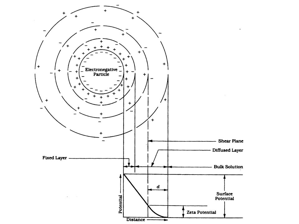
17. The formation of the electrical double layer (EDL) then occurs via attraction of oppositely charged counterions by the primary surface charge and then a diffusion of the counterions away from the surface. The counterions are mobile, the primary charge is not. The EDL development is schematically shown here:

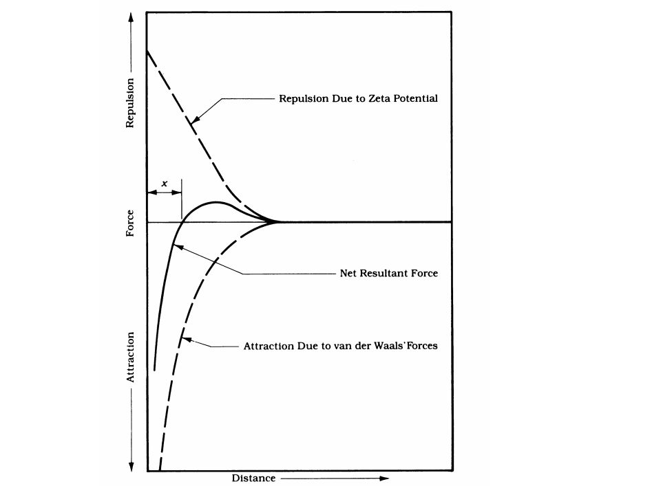
19. As a result of this EDL there is a net electrostatic repulsion/attraction developed between colloids. This net force is shown below:

21. The net resultant force is a result of: 1
The net resultant force is a result of: 1. attractive potential energy (mostly van der Waals forces), Va. These forces are very strong at short separation distances
2. repulsion potential energy (electrostatic forces), VR. (by Coulomb’s law).

22. The rate of agglomeration of colloids depends on the net resultant force between colloids. The higher the net repulsive force the less effective will be the coagulation. The basic goal of coagulation is to reduce the net repulsive force. We’ll discuss ways to do that, but first let’s look at ways to quantify the EDL via Zeta Potential and Electrophoretic mobility.

23. When colloids are subjected to an electrical field they will migrate generally toward the positive electrode of the field . They move because the inner part of the colloid (with higher charge density than the overall colloid) will respond to the field and leave the outer diffuse layer behind. The EDL actually shears at a plane and the potential (voltage) of the EDL at this shear plane is called the Zeta Potential, z.

24. The zeta potential represents the net charge between the primary charge and the counter charge in the EDL located between the surface and the shear plane. It’s with this charge that the colloid interacts with other colloids.

25. Electrophoretic mobility (EM) is used to quantify this potential
Electrophoretic mobility (EM) is used to quantify this potential. The velocity of the colloid is measured (by microscopic observation) in the presence of an electrical field and after performing a force balance on the colloid we can derive:

26. e = dielectric constant
= viscosity of surrounding fluid.
EM is the velocity (observed) of colloid movement divided by the voltage gradient. Generally units would be cm/sec per volts/cm.

27. Note that there is no way to know what the zeta potential should be to get effective coagulation, but in general lower ZP means better coagulation effectiveness.

28. Removal of Hydrophobic Colloids from the Aqueous Phase
Removal of hydrophobic colloids in water and wastewater treatment processes involves two steps:
·       

29. Destabilization (or Coagulation) - reduce the forces acting to keep the particles apart after they contact each other (i.e., lower repulsion forces).
Flocculation – process of bringing destabilized colloidal particles together to allow them to aggregate to a size where they will settle by gravity.

30. After coagulation /flocculation, gravity sedimentation, and sometimes filtration, are employed to remove the flocculated colloids.

31. Methods to Destabilize Colloids ( Coagulation Processes):
1. Double layer compression: This can be accomplished by addition of an indifferent electrolyte (charged ions with no specific attraction for colloid primary surface). Adding indifferent electrolyte increases the ionic strength of solution which has the effect of compressing the EDL. As the counterions are pushed closer to the surface the repulsion forces becomes easier to negate by van der Waals forces.

33. Charge on the added indifferent electrolyte is important according to the Schulze-Hardy rule that states the dosage for effective coagulation is logarithmically related to charge. For example the concentration of Na+, Ca2+ and Al3+ required for effective coagulation will vary in ratio of 1:10-2:10-3

34. With this type of coagulation can not get overdosing (as we will see later you can get with other types of coagulation). Also there is no relationship between colloid concentration and optimum dosage of coagulant. The same amount of indifferent electrolyte is required for low and high concentration of colloids. This means of coagulation is not very effective in water/wastewater treatment.

35. 2. Adsorption and Charge Neutralization: If charged (+) counterions have a specific affinity for the surface of the colloid (not merely electrostatic attraction) then adsorption of the counter-ion will reduce the primary charge of the colloid. This will reduce the net potential, y{r}, at any particular r thus making the attraction forces more effective. ZP is likely to be reduced also.

36. Counter-ions can be adsorbed by ion exchange, coordination bonding, van der Waals forces, repulsion of the coagulant by the aqueous phase (surface-active coagulant).

37. Characteristics of Adsorption/Neutralization:
Destabilize at lower concentration than indifferent electrolytes.
 Destabilization is a function of ion adsorptivity. Adsorptivity is a function of counter-ion size. Larger ions are not hydrated as easily as smaller ions so they are more easily adsorbed to lower solvent/ion attraction ( i.e., more surface active).

38. 3. Polymerized molecules are more easily adsorbed than non-polymerized species- related to (2).
4. Adsorption can result in overdosing with subsequent surface charge reversal.
5. Optimal dosage of coagulant is proportional to colloid concentration.—“stoichiometry of coagulation”.

39.   3. Adsorption and Interparticle bridging: In this case polymers, metal salt or synthetic organic types, specifically adsorb to surface, often charge neutralization occurs (Reaction 1 below), but further, other parts of the polymer adsorb to other colloids. This forms a polymer bridge as schematically shown below (Reaction 2). Using the definitions discussed above Reaction 1 represents "coagulation" and Reaction 2 represents "flocculation". There is stoichiometry of coagulation (dosage of coagulant is proportional to colloid concentration.

41. Adsorption is specific (usually chemical bonding), it is possible to adsorb negative or neutral polymers to the typically negative colloid surface.
Overdosing is possible. Basically the polymer covers the surface of the colloids without bridging to another colloid. This is shown in the following figure.

43. 4. Enmeshment in a precipitate (sweep floc): If metal salts, e. g
4. Enmeshment in a precipitate (sweep floc): If metal salts, e.g., Al2(SO4)3 , FeCl3 are added in sufficient quantities to exceed the solubility products of the metal hydroxide, oxide or, sometimes carbonates a “sweep floc” will form. Colloids will become enmeshed in the settling sweep floc and be removed from the suspension.

44. Because colloids can serve as a nucleation site for precipitating Al or Fe oxides the relationship between optimum coagulant dose (Al or Fe) and colloid concentration is often inverse. Also there is probably some primary charge neutralization and polymer bridging occurring simultaneously. There is evidence that the possibility of charge reversal is mitigated by the presence of SO42-.
SO42- is postulated to be adsorbed to the charge-reversed primary surface and the surface becomes negative again.

45. Metal salt chemistry as it relates to coagulation.
The primary metal salts used as coagulants are Al or Fe sulfate. How these salts work depends on the pH. We should look at the aqueous chemistry of these metals first.
Both Fe and Al are “hydrolyzing” metals. When dissolved, they try to push H+ out of the primary hydration shell. The degree to which this occurs depends on the pH.

46. For example for Al dissolved in water:
These monomers can combine to form polymers:
Such as Al3O4(OH)247+ or Al3(OH)45+

47. Similar reactions occur for Fe
Similar reactions occur for Fe. The speciation of both Al and Fe is highly pH dependent. The following graphs show how the Al and Fe species vary with pH.

50. In general, the lower the pH the higher the positive charge per Al or Fe species. Also the higher the pH the larger the dominant species and hence the greater the tendency to form polymers. This influences greatly how the coagulant will work.

51. For example, at low pH ( higher + charge per Al or Fe) the primary mode of coagulation is primary charge reduction. But since there is a higher charge per Al or Fe there is an increased risk of overdosing to get charge reversal. At higher pH get larger Al or Fe species up to polymers, but the charge per Al or Fe decreases. So at higher pH get more adsorption and bridging and then finally sweep floc (if the saturation concentration is reached).

52. Synthetic polymers are not as pH dependent and their mode of coagulation is primarily adsorption and bridging.

53. Dosing Strategies (for hydrolyzing metal salts)
Define zones of effectiveness:
Zone 1: Low dosage, insufficient coagulant added to produce destabilization.
Zone 2: Dosage sufficient to cause efficient and rapid destabilization
Zone 3: Dosage high enough to cause restabilization (charge reversal or polymer –foldback)
Zone 4: Dosage high enough to get sweep floc which results in good destabilization.

54. The dosages which result in these zones depends on the colloid concentration, often measured in terms of surface area Let’s look at 4 different values for S and see how the zones develop. S1 < S2 < S3 <S4.

56. Explanation:
At very low there is not enough particle-particle interaction to produce good destabilization and provide nuclei for the sweep floc to form. Therefore need high dosages. Restabilization is not a concern, since we are in the sweep-floc mode.

57. As increases into the 2 and levels there is sufficient colloid concentration to effect destabilization before sweep floc is reached. Note there is stoichiometry of coagulation and that it’s easier to restabilize at lower .

58. Finally at very high need lots of coagulant because of the large surface area. Although dosages may approach those of the sweep floc range, probably don’t get sweep floc because much of the coagulant is used by the colloids. In this scenario it’s almost impossible to overdose. Also we get stoichiometry of coagulation.
This information can be recompiled into the following chart:

60. This chart shows the coagulant dose required to get coagulation for various values. Note the stoichiometry of coagulation. Also note that for low a coagulant aid such as bentonite (a colloidal clay) can be added to increase to the point where we can get zone 2 coagulation instead of zone 4 coagulation. This saves on coagulant costs.

61. Since adding Al or Fe salts affects the pH and pH affects the speciation of Al and Fe it’s important to consider the following cases:
1. High Colloid, low alkalinity: The strategy here is to add coagulant and don’t worry about pH, the lower it falls the better because we are destabilizing by charge neutralization and the lower the pH the more charge neutralization we get from each Al or Fe added. There is no concern with overdosing because the colloidal surface area is too large.

62. 2. High colloid concentration, high alkalinity (often a situation encountered in sludge dewatering): The choices are to destabilize by adsorption/charge neutralization at neutral pH (because pH will probably stay near neutral even if large dosages of coagulant are applied. (Will need a larger dose at higher pH). Or elutriate (wash) the sludge to lower alkalinity Or add acid to lower pH. Economics dictate choice.

63. 3. Low colloid concentration , high alkalinity: For this case we can either destabilize by high dosage to give sweep floc or we can add coagulant aid such as bentonite to get destabilization at lower dosage.

64.   4. Low colloid concentration, low alkalinity:
This is the most difficult case and generally requires added alkalinity and bentonite. Sweep floc is difficult to form as pH drops and it’s easy to overdose at low pH and low .
Note that if PO4 is present Fe or Al will be consumed as FePO4 or AlPO4 before the metals act as coagulants. Must add 1/1 mole ratio of Al or Fe/PO4 to compensate for this consumption of Al or Fe.

65. JAR TESTS:
After the proper strategy is selected as described above, “jar tests” are performed. The jar test simulate the coagulation/flocculation process in a batch mode. A series of batch tests are run in which pH, coagulant type and dosage and coagulant aid are varied to get the optimal dosage (lowest residual turbidity). An economic analysis is performed to select these parameters.

66. Jar tests generally are performed using 6 one-liter samples of the water or wastewater to be treated. To these samples a range of coagulant (and possibly coagulant aid) dose is added (one sample is usually a blank). Immediately after the coagulant is added the samples are "flash mixed" for approximately one minute. The stirrer speed is then reduced to simulate a flocculation basin. Flocculation mode is generally maintained for about 20 minutes.

67. At the end of the flocculation period the stirrers are turned off and the floc is allowed to settle for one-half hour. After this settling period supernatant samples are drawn off from each sample and analyzed for turbidity and sometimes alkalinity and pH.

68. An actual gang-stirrer apparatus is shown in the figure below.

69. Typical results from a jar test series might look like:
Dose (mg/L)

70. Coagulation/Flocculation Tanks
The mechanics of coagulation and flocculation are accomplished in coagulation and flocculation tanks.

71. Coagulation is performed in a rapid-mix tank:
The objective of a rapid-mix tank is to destabilize the colloids. Depending on the coagulant type and dosage of coagulant the rapid-mix tank provides a reactor to:

72. form polymers if Al or Fe are used as coagulants
evenly distribute Fe or Al polymers to colloidal surfaces
3) form sweep floc (Al or Fe)
4) evenly distribute polymers to surface of colloids if organic polymers (synthetic) are used.

73. Mixing Levels:
Mixing intensity and residence time determine whether the stated goals will be met.
To determine mixing intensity define as the average shear intensity (mean velocity gradient) in the rapid-mix tank.
The Camp-Stein equation is often used to compute this , however it is an equation which is based on laminar flow -- a case seldom found in rapid-mix or flocculation basins so it’s an “average” approximation.

74. The Camp-Stein equation is :
= power dissipation (mixer power transferred to bulk fluid)
V = volume of reactor
m = dynamic viscosity

75. should have units of 1/time.
The units for P, V and m have to be consistent.

76. This is an average velocity gradient over the entire basin
This is an average velocity gradient over the entire basin. There is a much higher intensity at the tips of the mixer blades. This is where most of the mixing occurs in coagulation and flocculation. The figure shown below demonstrates typical distribution of shear in a back-mixed reactor. In spite of this heterogeneous distribution, overall the average velocity gradient is a good operational value for controlling and quantifying mixing.

78. Continuing, for rapid-mix tanks:
For backmix (external mixing) reactors:
= per sec.
q = 1 min.

79. Sometimes in-line or static mixers are used for rapid-mixing
Sometimes in-line or static mixers are used for rapid-mixing. This type of mixer is illustrated here:

80. For in-line mixers for effective coagulation:
= per sec.
q = < 10 sec.
These parameters are not adjustable and are set by the manufacturer.

81. Flocculation:
Rapid mix (coagulation ) is followed by flocculation where there is slow, enhanced contact between destabilized (coagulated) particles. Flocculation basins are used to promote growth of the destabilized floc by promoting particle-particle contact.
There are two modes of particle-particle contact.

82. Perikinetic flocculation:
Thermal activity or Brownian motion is responsible for colloid collisions in the case of perikinetic flocculation. Smoluchowski theory can be used to predict rate of reduction of particle (colloid) number with time, Jpk, via perikinetic flocculation.

83. For particles of equal size:
N = particle number concentration
m = dynamic viscosity (0.01 g/cm-sec)
kT = x ergs
a = collision efficiency (0 - 1)

84. Integration of this rate equation (for a batch reactor) over time gives:

85. Orthokinetic Flocculation
In this case there is an external mixing source which promotes particle-particle contact. The rate of colloid number decrease, Jok, is given by:
d = particle diameter.

86. Evaluation of orthokinetic flocculation rate is difficult because d changes with time. This problem can be handled in the following manner:
First define:
W = volume of colloids/total volume of suspension. is essentially constant during flocculation. (assuming there is no settling of floc particles in the flocculation basin)

87. Assuming equal diameter spherical colloids:
At time = 0
N0 is initial colloid number concentration (number/volume of suspension).

88. Then:

89. Integration for a batch process yields:

90. Example calculation of W:
A sample contains 200 mg/L of colloids. The average density of these colloids is 1.1 g/cm3.

91. Under flocculation (orthokinetic) the particles will increase in size until the floc particles become large enough to be subjected to shear forces which disrupt the particles. These shear forces increase the particle numbers, i.e., they work in the opposite direction of flocculation. One model for the floc break-up is given by:

92. K’B = floc breakup coefficient (must be determined experimentally) [time/volume]
Then:

93. Integration over time yields:
Or:

94. For a continuous flow, completely mixed, flocculation tank at steady-state:

95. The time required to reach a certain number reduction can be calculated with these equations. The form of the equation is more important than the magnitude of the coefficients (which are inherently difficult to quantify) .

96. To meet the objective of increasing floc size to the point where they will settle by gravity flocculation basins are designed for more gentle agitation and longer contact time then would be found in a rapid mix tank. Often these tanks are designed with tapered flocculation so that the shear environment is reduced in intensity as the floc particles grow.

97. Orthokinetic flocculation equations are often used to predict performance of flocculation basins.
The major design parameters for these basins are (as controlled by mixing input) and q (as controlled by tank volume). Typical design for a flocculation basin would be:

98. Typical design for a tapered flocculation basin would be:

99. For tapered flocculation systems varies in each reactor, but q is generally constant. The goal is to maintain total q to be in the recommended range ( ).
We also need to maintain a level of mixing to prevent sedimentation in the basins. This level is about = 10 – 15 sec-1 .

100. To predict the effectiveness of the flocculation basin we need to quantify a and W.
a and are difficult to determine although order of magnitude estimates can easily be made:
For example:
a = 0.1,
W =

101. Neither of these parameters are controlled by the flocculation process (a is basically controlled by the coagulation process). q and can be controlled to compensate for W and a.
Presumably the best flocculation performance occurs when N/N0 is the lowest.

103. Some typical flocculation basins are shown here: