Download presentation
Presentation is loading. Please wait.

1
X-ray Astrostatistics Bayesian Methods in Data Analysis Aneta Siemiginowska Vinay Kashyap and CHASC Jeremy Drake, Nov.2005

2
X-ray Astrostatistics Bayesian Methods in Data Analysis Aneta Siemiginowska Vinay Kashyap and CHASC Jeremy Drake, Nov.2005

3
CHASC: California-Harvard Astrostatistics Collaboration http://hea-www.harvard.edu/AstroStat/ History: why this collaboration? Regular Seminars: each second Tuesday at the Science Center Participate in SAMSI workshop => Spring 2006 Participants: HU Statistics Dept., Irvine UC, and CfA astronomers Topics related mostly to X-ray astronomy, but also sun-spots! Papers: MCMC for X-ray data, Fe-line and F-test issues, EMC2, hardness ratio and line detection Algorithms are described in the papers => working towards public release Stat: David van Dyk, Xiao-Li Meng, Taeyoung Park, Yaming Yu, Rima Izem Astro: Alanna Connors, Peter Freeman, Vinay Kashyap, Aneta Siemiginowska Andreas Zezas, James Chiang, Jeff Scargle

4
X-ray Data Analysis and Statistics Different type analysis: Spectral, image, timing. XSPEC and Sherpa provide the main fitting/modeling environments X-ray data => counting photons: -> normal - Gaussian distribution for high number of counts, but very often we deal with low counts data Low counts data (< 10) => Poisson data and 2 is not appropriate! Several modifications to 2 have been developed: Weighted 2 (.e.g. Gehrels 1996) Formulation of Poisson Likelihood ( C follows for N>5) Cash statistics: (Cash 1979) C-statistics - goodness-of-fit and background (in XSPEC, Keith Arnaud)
 => Poisson data and 2 is not appropriate. Several modifications to 2 have been developed: Weighted 2 (.e.g. Gehrels 1996) Formulation of Poisson Likelihood ( C follows for N>5) Cash statistics: (Cash 1979) C-statistics - goodness-of-fit and background (in XSPEC, Keith Arnaud).")
5
Steps in Data Analysis Obtain data - observations! Reduce - processing the data, extract image, spectrum etc. Analysis - Fit the data Conclude - Decide on Model, Hypothesis Testing! Reflect

6
Hypothesis Testing How to decide which model is better? A simple power law or blackbody? A simple power law or continuum with emission lines? Statistically decide: how to reject a simple model and accept more complex one? Standard (Frequentist!) Model Comparison Tests: Goodness-of-fit Maximum Likelihood Ratio test F-test
 Model Comparison Tests: Goodness-of-fit Maximum Likelihood Ratio test F-test.")
7
Steps in Hypothesis Testing - I

8
Steps in Hypothesis Testing - II Two model Mo (simpler) and M1 (more complex) were fit to the data D; Mo => null hypothesis. Construct test statistics T from the best fit of two models: e.g. = Determine each sampling distribution for T statistics, e.g. p(T | Mo) and p(T | M1) Determine significance => Reject Mo when p (T | Mo) < Determine the power of the test => probability of selecting Mo when M1 is correct p(T|Mo) p(T|M1)
 and p(T | M1) Determine significance => Reject Mo when p (T | Mo) < Determine the power of the test => probability of selecting Mo when M1 is correct p(T|Mo) p(T|M1).")
9
Conditions for LRT and F-test The two models that are being compared have to be nested: broken power law is an example of a nested model BUT power law and thermal plasma models are NOT nested The null values of the additional parameters may not be on the boundary of the set of possible parameter values: continuum + emission line -> line intensity = 0 on the boundary References Freeman et al 1999, ApJ, 524, 753 Protassov et al 2002, ApJ 571, 545

10
Simple Steps in Calibrating the Test: 1.Simulate N data sets (e.g. use fakeit in Sherpa or XSPEC): => the null model with the best-fit parameters (e.g. power law, thermal) => the same background, instrument responses, exposure time as in the initial analysis 2.(A) Fit the null and alternative models to each of the N simulated data sets and (B) compute the test statistic: T LRT = -2log [L( |sim)/L( |sim)] best fit parameters T F = 3.Compute the p-value - proportion of simulations that results in a value of statistic (T) more extreme than the value computed with the observed data. p-value = (1/N) * Number of [ T(sim) > T(data) ]
: => the null model with the best-fit parameters (e.g. power law, thermal) => the same background, instrument responses, exposure time as in the initial analysis 2.(A) Fit the null and alternative models to each of the N simulated data sets and (B) compute the test statistic: T LRT = -2log [L( |sim)/L( |sim)] best fit parameters T F = 3.Compute the p-value - proportion of simulations that results in a value of statistic (T) more extreme than the value computed with the observed data. p-value = (1/N) * Number of [ T(sim) > T(data) ].")
11
Simulation Example M0 - power law M1 - pl+narrow line M2 - pl+broad line M3 - pl+absorption line M0/M1 M0/M2M0/M3 Comparison between p-value And significance in the distribution =0.05 Reject Null Accept Null

12
Simulation Example M0 - power law M1 - pl+narrow line M2 - pl+broad line M3 - pl+absorption line M0/M1 M0/M2M0/M3 Comparison between p-value And significance in the distribution =0.05 Reject Null Accept Null

13
Bayesian Methods use Bayesian approach - max likelihood, priors, posterior distribution - to fit/find the modes of the posterior (best fit parameters) Simulate from the posterior distribution, including uncertainties on the best-fit parameters, Calculate posterior predictive p-values Bayes factors: direct comparison of probabilities P(M1)/P(Mo)
 Simulate from the posterior distribution, including uncertainties on the best-fit parameters, Calculate posterior predictive p-values Bayes factors: direct comparison of probabilities P(M1)/P(Mo)")
14
CHASC Projects at SAMSI 2006 Source and Feature detection Working group Issues in Modeling High Counts Data Image reconstructions (e.g. Solar data) Detection and upper limits in high background data (GLAST) Smoothed/unsharp mask images - significance of features Issues in Low Counts Data Upper limits Classification of Sources - point source vs. extended Poisson data in the presence of Poisson Background Quantification of uncertainty and Confidence Other Projects in Town: Calibration uncertainties in X-ray analysis Emission Measure model for X-ray spectroscopy (Log N - Log S) model in X-ray surveys
 Detection and upper limits in high background data (GLAST) Smoothed/unsharp mask images - significance of features Issues in Low Counts Data Upper limits Classification of Sources - point source vs. extended Poisson data in the presence of Poisson Background Quantification of uncertainty and Confidence Other Projects in Town: Calibration uncertainties in X-ray analysis Emission Measure model for X-ray spectroscopy (Log N - Log S) model in X-ray surveys.")
15
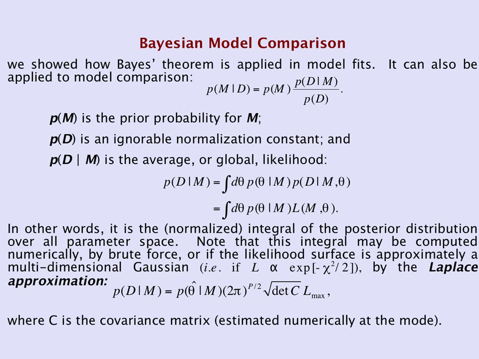
Bayesian Model Comparison To compare two models, a Bayesian computes the odds, or odd ratio: where B 10 is the Bayes factor. When there is no a priori preference for either model, B 10 = 1 of one indicates that each model is equally likely to be correct, while B 10 ≥ 10 may be considered sufficient to accept the alternative model (although that number should be greater if the alternative model is controversial).
..")
17
Model Comparison Tests A model comparison test statistic T is created from the best-fit statistics of each fit; it is sampled from a probability distribution p(T). The test significance is defined as the integral of p(T) from the observed value of T to infinity. The significance quantifies the probability that one would select the more complex model when in fact the null hypothesis is correct. A standard threshold for selecting the more complex model is significance < 0.05 (the "95% criterion" of statistics). p(T|Mo) p(T|M1)
 from the observed value of T to infinity. The significance quantifies the probability that one would select the more complex model when in fact the null hypothesis is correct. A standard threshold for selecting the more complex model is significance < 0.05 (the 95% criterion of statistics). p(T|Mo) p(T|M1).")
Similar presentations


 Methods Nelson Christensen Carleton College LIGO-G020104-00-Z.>")


 1 Gamma-ray Large Area Space Telescope Challenges.>")


: Alternative Hypothesis (H 1 ): a statistical analysis used to decide which of two competing.>")


