1. Introduction to M ATLAB 2 Graphics Ian Brooks Institute for Climate & Atmospheric Science School of Earth & Environment i.brooks@see.leeds.ac.uk

2. GRAPHICS Basic Plotting –Linetypes, markers, colours, etc Subplots – creating multiple axes on a single figure Annotating figures – titles, labels, legends Editing figure properties Other plotting functions

3. Basic Plotting Commands figure : creates a new figure window plot(x) : plots line graph of x vs index number of array plot(x,y) : plots line graph of x vs y plot(x,y,'r--') : plots x vs y with linetype specified in string : 'r' = red, 'g'=green, etc for a limited set of basic colours.

4. Plot(x,y,…properties) Plot(x,y,cml) – plot with a basic colour-marker- line combination (cml) –‘ro-’, ‘g.-’, ‘cv--‘ –Basic colours : r, g, b, k, y, c, m –Basic markers : ‘o’, ‘v’, ‘^’, ’ ’, ‘.’, ‘p’, ‘+’, ‘*’, ‘x’, ‘s’, ‘h’, ‘none’ –Linetypes : ‘-’, ’--‘, ‘-.’, ‘:’, ‘none’

5. More detailed plot options can be specified through the use of property:value pairs –Plot(x,y,’o-’,’property’,value) ‘property’ is always a string naming the propery, value may be a number, array, or string, depending on the property type: ‘color’ : [R G B] - color (american spelling!) is specified with a [red green blue] value array, each in range 0-1. [1 0 0] – pure red [1 0. 0.5 0] – orange

6. –‘linewidth’ : specified as a single number. Default = 0.5 –‘linestyle’ : any of line type strings - ‘-’,’:’,etc –‘marker’ : any of marker strings – ‘v’, ’o’, etc –‘markersize’ : number, default = 6 –‘markeredgecolor’ : color string ‘r’, ‘g’, or [R G B] value for the line defining edge of marker –‘markerfacecolor’ : color string or [R G B] for inside of marker (can be different from edge) Can add any number of property:value pairs to a plot command: >> Plot(x,y,’prop1’,value1,’prop2’,value2,..)

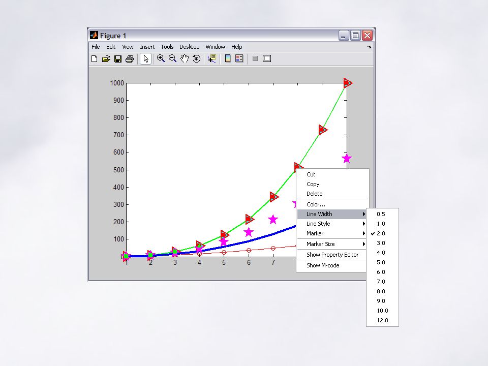
9. Property Editor — Axis Tree of objects Edited objects Help for object

10. GUI property browser & editor Access from the figure’s view menu

11. Subplots subplot(m,n,p) : create a subplot in an array of axes >> subplot(2,3,1); >> subplot(2,3,4); m n P=1 P=2 P=3 P=4

12. Adding Text to Figures Basic axis labels and title can be added via convenient functions: >> xlabel('x-axis label text') >> ylabel('y-axis label text') >> title('title text') Legends for line or symbol types are added via the legend function: >> legend('line 1 caption','line 2 caption',…) Legend labels are given in the order lines were plotted

13. ‘Handle’ Graphics MATLAB uses a hierarchical graphics model –Graphics objects organised according to their dependencies: e.g. lines must be plotted on axes, axes must be positioned on figures –Every object has a unique identifier, or handle Handles are returned by the creating function –ax = subplot(3,2,n) –H = plot(x,y) Handles can be used to identify an object in order to inspect (get) or modify (set) its properties at any time

14. root figure axesUI-controlUI-menuUI-contextmenu linelightimagepatchsurfacerectangletext Object Hierarchy The computer desktop Figure window Objects at any level are considered to be ‘children’ of their ‘parent’ object.

15. Properties of an object with handle H, can be inspected/modified by: >> value = get(H,'propertyname') >> set(H,'propertyname',value) All property values echoed to screen by: >> get(H) 3 useful functions: –gcf : get current figure – returns handle of current figure –gca : get current axes – returns handle of current axes –gco : get current object – returns handle of current object Can use these directly, instead of the handle

16. Current object is last created (usually), or last object clicked on with mouse. >> pp = get(gca,'position') pp = 0.1300 0.1100 0.7750 0.8150 >> set(gca,'position',pp+[0 0.1 0 -0.1]) The code above first gets the position of the current axes – location of bottom left corner (x 0, y 0 ), width (dx) and height (dy) (in normalised units) – then resets the position so that the axes sit 0.1 units higher on the page and decreases their height by 0.1 units.

17. Other plotting functions Matlab has many plotting functions – we will use a simple data set representing a surface to try these out. Enter the command peaks z = 3*(1-x).^2.*exp(-(x.^2) - (y+1).^2)... - 10*(x/5 - x.^3 - y.^5).*exp(-x.^2-y.^2)... - 1/3*exp(-(x+1).^2 - y.^2) Peaks sets up a regular x and y grid, and defines the function z given above.

18. >> peaks; Peaks is an example function, useful for demonstrating 3D data, contouring, etc. Figure above is its default output. P=peaks; - return data matrix for replotting…

19. >> P = peaks; - save output of peaks in P >> contour(P) - contour P using default contour values x and y axes are simply the row and column numbers

20. >> contour(P,[-9:0.5:9]) – contour with specified contour values.

21. >> [C,h]=contour(P); - capture Contour value and handle >> clabel(C,h); - clabel function adds labels

22. >> [x,y,P] = peaks; >> contour(x,y,P,[-9:9]) x and y axes are true values

23. >> contourf(P,[-9:0.5:9]); - filled contour function >> colorbar - add colour scale

24. Pseudocolour plots An alternative to contouring – provides a continuous colour-mapped 2D data field pcolor(Z) : plot pseudocolour plot of Z pcolor(X,Y,Z) : plot of Z on grid X,Y shading faceted | flat | interp : set shading option –faceted : show edge lines (default) –flat : don't show edge lines –interp : colour is linearly interpolated to give smooth variation

25. >> pcolor(P)>> shading flat >> shading interp Data points are at vertices of grid, colour of facet indicates mean value of surrounding vertices. Colours are selected by interpolating data range into a colormap

26. >> pcolor(P);shading flat >> hold on >> contour(P,[1:9],'k') >> contour(P,[-9:-1],'k--') >> contour(P,[0 0],'k','linewidth',2) >> colorbar

27. colormaps Surfaces are coloured by scaling the data range to the current colormap. A colormap applies to a whole figure. Several predefined colormaps exist ('jet' (the default), 'warm','cool','copper','bone','hsv'). Select one with >> colormap mapname >> colormap('mapname') The current colormap can be retrieved with >> map=colormap

28. >> colormap cool

29. >> caxis([0 8]) - caxis function sets the [min max] limits of >> colorbar the colour scale. Need to refresh colourbar

30. Colormaps are simply 3-column matrices of arbitrary length (default = 64 rows). Each row contains the [RED GREEN BLUE] components of the colour required, specified on a 0  1 scale. e.g. >> mymap =[ 0 0 0.1 0 0.1 0.2 0.1 0.2 0.3...... ] >> colormap(mymap)

31. Specialized Plotting Routines

32. Specialized Plotting Routines (Continued)

33. Load jun07_all_5km_means.mat Variables: mlat, mlon- latitude & longitude of measurements mT- mean air temperature msst- mean sea surface temperature mu, mv- mean wind components to east (x) and north (y) mws- mean wind speed Plot the different variables to get a feel for range of values and relationships between them. Plot positions of the points - geographical locations

34. >> load jun07_all_5km_means.mat >> who Your variables are: mT mlat mlon msst mu mv >> plot(mlon,mlat,'o‘)

35. >> plot(mlon,mlat,'o') >> hold on >> quiver(mlon,mlat,mu,mv)

36. Randomly distributed data can’t be used with contour, pcolor, surf, etc…data needs to be on a regular grid. Use meshgrid to generate arrays of x and y on a regular grid. [XX,YY] = meshgrid([-125.2:0.05:-124],[39.9:0.05:40.8]); Use griddata to interpolate mu and mv onto the XX,YY grid … use system help to check usage X-values requiredY-values required X and Y grids

37. >> [XX,YY] = meshgrid([-125.2:0.05:-124],[39.9:0.05:40.8]); >> gmws = griddata(mlon,mlat,mws,XX,YY); >> pcolor(XX,YY,gmws); shading flat; >> hbar = colorbar; >> hold on >> h1 = plot(mlon,mlat,'ko');

38. >> gu=griddata(mlon,mlat,mu,XX,YY); >> gv=griddata(mlon,mlat,mv,XX,YY); >> quiver(XX,YY,gu,gv,'k-'); >> set(h1,'markeredgecolor','r','markersize',5)

39. >> set(gca,'linewidth',2,'fontweight','bold') >> xlabel('Longitude'); ylabel('latitude') >> set(hbar,'linewidth',2,'fontweight','bold') >> set(get(hbar,'xlabel'),'string','(m s^{-1})','fontweight','bold') >> xlabel('Longitude'); ylabel('latitude') >> title('CW96 : June 07 : 30m wind field') >> load mendocinopatch.mat >> patch(mendocinopatch(:,1),mendocinopatch(:,2),[0.9 0.9 0.9])

40. Printing From file menu: –‘print’ to send to a printer –Export to export to a file (gif, png, jpg, eps,…) Better to use command line > print filename.EXT -dEXT File-type extension ‘png’, ‘ps’, ‘.eps’ appropriate to file type you want Instruction to print engine to select file type (same format as a linux print destination)

41. > print myfigure.png -dpng > print myfigure.png –dpng –r300 -rNNN option specifies print resolution to NNN dpi

42. Common print file types –.ps- postscript (full page) –.eps- encapsulated postscript (embeddable, infinitely scalable vector graphic – best for publication) –.png- portable network graphic – best bitmap image option –.jpg- JPEG image NEVER USE THIS!

43. . png.jpg JPEG format is designed for photographic images with continuously varying tone. Hard edges suffer compression artefacts – distortions – ugly, and can make text impossible to read

44. .fig files > hgsave(gcf,’filename.fig’) Saves the current figure to a.fig file – this is a complete description of the figure as a set of matlab handle-graphics objects. Can reload the figure to make edits later > hgload(‘filename.fig’)