Download presentation
Presentation is loading. Please wait.

1
Friday: 2-3:15pm BY 510 make-up class Today: 1. Online search 2. Planning in Belief-space

2
Online Search Online Search (with the knowledge of transition model) To avoid planning for all contingencies.. Qn: How worse off are you compared to someone who took the model into account? Competitive Ratio “Adventure is just Failure to Plan” Online Search (in the absence of transition model) All you can do is act, learn the model, use it to act better Cannot use search methods that require shifting branches Depth-First okay Hill-Climbing okay—but not random- restart. Random-walk okay Need to learn the model Taboo list; LRTA*, Reinforcement learning -- as against “Offline” search. Agent interleaves search and execution. Necessary when there is no model. May be useful when the model is complex (non-determinism etc) Where did you see online search in 471? Is it full or no model?
 All you can do is act, learn the model, use it to act better Cannot use search methods that require shifting branches Depth-First okay Hill-Climbing okay—but not random- restart. Random-walk okay Need to learn the model Taboo list; LRTA*, Reinforcement learning -- as against Offline search. Agent interleaves search and execution. Necessary when there is no model. May be useful when the model is complex (non-determinism etc) Where did you see online search in 471. Is it full or no model .")
4
Online Search as a Hammer that can hit many nails.. If you have no model, you will need online search Since only by exploring you can figure out the model ..and as you learn part of the model, you are stuck with the exploration/exploitation tradeoff If you have a model, but you are too lazy to use it, you need online search Limited contingency planning; planning and replanning; online stochastic planning If you have no time to reason, you will need to do online search E.g. dynamic and semi-dynamic scenarios Online search doesn’t mean “no need whatsoever to think” --Trick is to use partial model (either learned or excerpted)
.")
6
BELIEF-SPACE PLANNING

7
Representing Belief States

8
What happens if we restrict uncertainty? If initial state uncertainty can be restricted to the status of single variables (i.e., some variables are “unknown” the rest are known), then we have “conjunctive uncertainty” With conjunctive uncertainty, we only have to deal with 3 n belief states (as against 2^(2 n )) Notice that this leads to loss of expressiveness (if, for example, you know that in the initial state one of P or Q is true, you cannot express this as a conjunctive uncertainty Notice also the relation to “goal states” in classical planning. If you only care about the values of some of the fluents, then you have conjunctive indifference (goal states, and thus regression states, are 3 n ). Not caring about the value of a fluent in the goal state is a boon (since you can declare success if you reach any of the complete goal states consistent with the partial goal state; you have more ways to succeed) Not knowing about the value of a fluent in the initial state is a curse (since you now have to succeed from all possible complete initial states consistent with the partial initial state)
, then we have conjunctive uncertainty With conjunctive uncertainty, we only have to deal with 3 n belief states (as against 2^(2 n )) Notice that this leads to loss of expressiveness (if, for example, you know that in the initial state one of P or Q is true, you cannot express this as a conjunctive uncertainty Notice also the relation to goal states in classical planning. If you only care about the values of some of the fluents, then you have conjunctive indifference (goal states, and thus regression states, are 3 n ). Not caring about the value of a fluent in the goal state is a boon (since you can declare success if you reach any of the complete goal states consistent with the partial goal state; you have more ways to succeed) Not knowing about the value of a fluent in the initial state is a curse (since you now have to succeed from all possible complete initial states consistent with the partial initial state).")
9
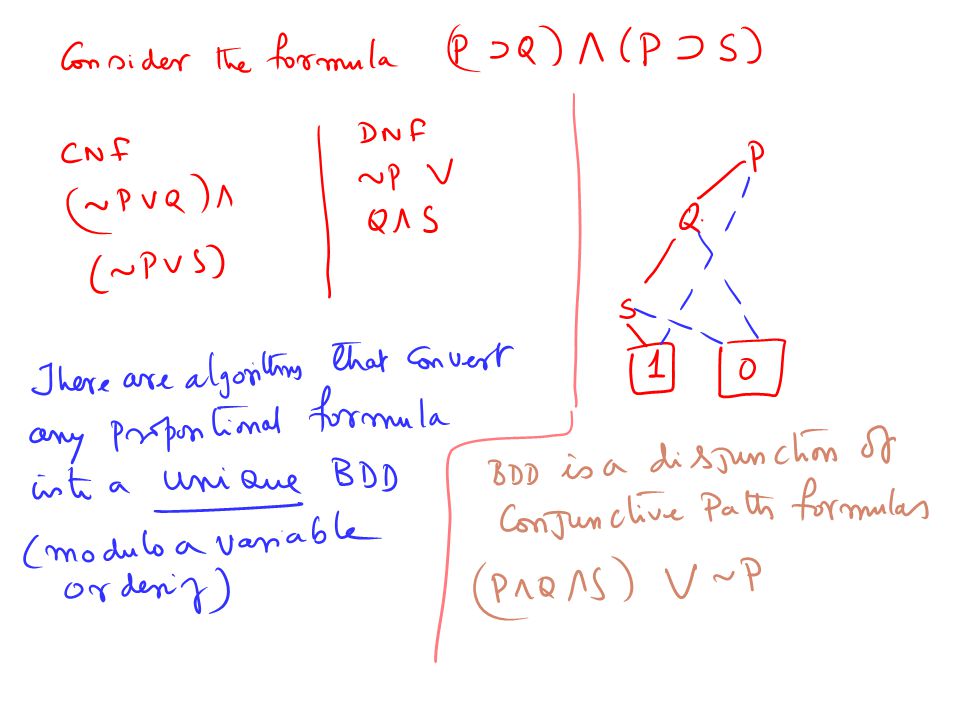
Belief State Rep (cont) Belief space planners have to search in the space of full propositional formulas!! In contrast, classical state-space planners search in the space of interpretations (since states for classical planning were interpretations). Several headaches: Progression/Regression will have to be done over all states consistent with the formula (could be exponential number). Checking for repeated search states will now involve checking the equivalence of logical formulas (aaugh..!) To handle this problem, we have to convert the belief states into some canonical representation. We already know the CNF and DNF representations. There is another one, called Ordered Binary Decision Diagrams that is both canonical and compact OBDD can be thought of as a compact representation of the DNF version of the logical formula
. Several headaches: Progression/Regression will have to be done over all states consistent with the formula (could be exponential number). Checking for repeated search states will now involve checking the equivalence of logical formulas (aaugh..!) To handle this problem, we have to convert the belief states into some canonical representation. We already know the CNF and DNF representations. There is another one, called Ordered Binary Decision Diagrams that is both canonical and compact OBDD can be thought of as a compact representation of the DNF version of the logical formula.")
10
Effective representations of logical formulas Checking for repeated search states will now involve checking the equivalence of logical formulas (aaugh..!) To handle this problem, we have to convert the belief states into some canonical representation. We already know the CNF and DNF representations. These are normal forms but are not canonical Same formula may have multiple equivalent CNF/DNF representations There is another one, called Reduced Ordered Binary Decision Diagrams that is both canonical and compact ROBDD can be thought of as a compact representation of the DNF version of the logical formula

13
Belief State Search: An Example Problem Initial state: M is true and exactly one of P,Q,R are true Goal: Need G Actions: A1: M P => K A2: M Q => K A3: M R => L A4: K => G A5: L => G Init State Formula: [(p & ~q & ~r)V(~p&q&~r)V(~p&~q&r)]&M DNF: [M&p&~q&~r]V[M&~p&~q&~r]V[M&~p&~q&r] CNF: (P V Q V R) & (~P V ~Q) &(~P V ~R) &(~Q V ~R) & M DNF good for progression (clauses are partial states) CNF good For regression Plan: ??
![Belief State Search: An Example Problem Initial state: M is true and exactly one of P,Q,R are true Goal: Need G Actions: A1: M P => K A2: M Q => K A3: M R => L A4: K => G A5: L => G Init State Formula: [(p & ~q & ~r)V(~p&q&~r)V(~p&~q&r)]&M DNF: [M&p&~q&~r]V[M&~p&~q&~r]V[M&~p&~q&r] CNF: (P V Q V R) & (~P V ~Q) &(~P V ~R) &(~Q V ~R) & M DNF good for progression (clauses are partial states) CNF good For regression Plan:](http://images.slideplayer.com/12/3378732/slides/slide_13.jpg "Belief State Search: An Example Problem Initial state: M is true and exactly one of P,Q,R are true Goal: Need G Actions: A1: M P => K A2: M Q => K A3: M R => L A4: K => G A5: L => G Init State Formula: [(p & ~q & ~r)V(~p&q&~r)V(~p&~q&r)]&M DNF: [M&p&~q&~r]V[M&~p&~q&~r]V[M&~p&~q&r] CNF: (P V Q V R) & (~P V ~Q) &(~P V ~R) &(~Q V ~R) & M DNF good for progression (clauses are partial states) CNF good For regression Plan:")
14
Progression & Regression Progression with DNF The “constituents” (DNF clauses) look like partial states already. Think of applying action to each of these constituents and unioning the result Action application converts each constituent to a set of new constituents Termination when each constituent entails the goal formula Regression with CNF Very little difference from classical planning (since we already had partial states in classical planning). THE Main difference is that we cannot split the disjunction into search space Termination when each (CNF) clause is entailed by the initial state
. THE Main difference is that we cannot split the disjunction into search space Termination when each (CNF) clause is entailed by the initial state.")
15
Progression Example

16
Regression Search Example Actions: A1: M P => K A2: M Q => K A3: M R => L A4: K => G A5: L => G Initially: (P V Q V R) & (~P V ~Q) & (~P V ~R) & (~Q V ~R) & M Goal State: G G (G V K) (G V K V L) A4 A1 (G V K V L V P) & M A2 A5 A3 G or K must be true before A4 For G to be true after A4 (G V K V L V P V Q) & M (G V K V L V P V Q V R) & M Each Clause is Satisfied by a Clause in the Initial Clausal State -- Done! (5 actions) Initially: (P V Q V R) & (~P V ~Q) & (~P V ~R) & (~Q V ~R) & M Clausal States compactly represent disjunction to sets of uncertain literals – Yet, still need heuristics for the search (G V K V L V P V Q V R) & M Enabling precondition Must be true before A1 was applied
 Initially: (P V Q V R) & (~P V ~Q) & (~P V ~R) & (~Q V ~R) & M Clausal States compactly represent disjunction to sets of uncertain literals – Yet, still need heuristics for the search (G V K V L V P V Q V R) & M Enabling precondition Must be true before A1 was applied.")
17
Symbolic model checking: The bird’s eye view Belief states can be represented as logical formulas (and “implemented” as BDDs ) Transition functions can be represented as 2-stage logical formulas (and implemented as BDDs) The operation of progressing a belief state through a transition function can be done entirely (and efficiently) in terms of operations on BDDs Read Appendix C before next class (emphasize C.5; C.6)
 Transition functions can be represented as 2-stage logical formulas (and implemented as BDDs) The operation of progressing a belief state through a transition function can be done entirely (and efficiently) in terms of operations on BDDs Read Appendix C before next class (emphasize C.5; C.6)")
18
Sensing: General observations Sensing can be thought in terms of Speicific state variables whose values can be found OR sensing actions that evaluate truth of some boolean formula over the state variables. Sense(p) ; Sense(pV(q&r)) A general action may have both causative effects and sensing effects Sensing effect changes the agent’s knowledge, and not the world Causative effect changes the world (and may give certain knowledge to the agent) A pure sensing action only has sensing effects; a pure causative action only has causative effects.
 ; Sense(pV(q&r)) A general action may have both causative effects and sensing effects Sensing effect changes the agent’s knowledge, and not the world Causative effect changes the world (and may give certain knowledge to the agent) A pure sensing action only has sensing effects; a pure causative action only has causative effects..")
19
Sensing at Plan Time vs. Run Time When applied to a belief state, AT RUN TIME the sensing effects of an action wind up reducing the cardinality of that belief state basically by removing all states that are not consistent with the sensed effects AT PLAN TIME, Sensing actions PARTITION belief states If you apply Sense-f? to a belief state B, you get a partition of B 1 : B&f and B 2 : B&~f You will have to make a plan that takes both partitions to the goal state Introduces branches in the plan If you regress two belief state B&f and B&~f over a sensing action Sense-f?, you get the belief state B

21
If a state variable p Is in B, then there is some action A p that Can sense whether p is true or false If P=B, the problem is fully observable If B is empty, the problem is non observable If B is a subset of P, it is partially observable Note: Full vs. Partial observability is independent of sensing individual fluents vs. sensing formulas. (assuming single literal sensing)
.")
22
Full Observability: State Space partitioned to singleton Obs. Classes Non-observability: Entire state space is a single observation class Partial Observability: Between 1 and |S| observation classes

24
Hardness classes for planning with sensing Planning with sensing is hard or easy depending on: (easy case listed first) Whether the sensory actions give us full or partial observability Whether the sensory actions sense individual fluents or formulas on fluents Whether the sensing actions are always applicable or have preconditions that need to be achieved before the action can be done
 Whether the sensory actions give us full or partial observability Whether the sensory actions sense individual fluents or formulas on fluents Whether the sensing actions are always applicable or have preconditions that need to be achieved before the action can be done")
25
A Simple Progression Algorithm in the presence of pure sensing actions Call the procedure Plan(B I,G,nil) where Procedure Plan(B,G,P) If G is satisfied in all states of B, then return P Non-deterministically choose: I. Non-deterministically choose a causative action a that is applicable in B. Return Plan(a(B),G,P+a) II. Non-deterministically choose a sensing action s that senses a formula f (could be a single state variable) Let p’ = Plan(B&f,G,nil); p’’=Plan(B&~f,G,nil) /*B f is the set of states of B in which f is true */ Return P+(s?:p’;p’’) If we always pick I and never do II then we will produce conformant Plans (if we succeed).
,G,P+a) II. Non-deterministically choose a sensing action s that senses a formula f (could be a single state variable) Let p’ = Plan(B&f,G,nil); p’’=Plan(B&~f,G,nil) /*B f is the set of states of B in which f is true */ Return P+(s :p’;p’’) If we always pick I and never do II then we will produce conformant Plans (if we succeed)..")
26
Very simple Example A1 p=>r,~p A2 ~p=>r,p A3 r=>g O5 observe(p) Problem: Init: don’t know p Goal: g Plan: O5:p?[A1 A3][A2 A3] Notice that in this case we also have a conformant plan: A1;A2;A3 --Whether or not the conformant plan is cheaper depends on how costly is sensing action O5 compared to A1 and A2
![Very simple Example A1 p=>r,~p A2 ~p=>r,p A3 r=>g O5 observe(p) Problem: Init: don’t know p Goal: g Plan: O5:p [A1 A3][A2 A3] Notice that in this case we also have a conformant plan: A1;A2;A3 --Whether or not the conformant plan is cheaper depends on how costly is sensing action O5 compared to A1 and A2](http://images.slideplayer.com/12/3378732/slides/slide_26.jpg "Very simple Example A1 p=>r,~p A2 ~p=>r,p A3 r=>g O5 observe(p) Problem: Init: don’t know p Goal: g Plan: O5:p [A1 A3][A2 A3] Notice that in this case we also have a conformant plan: A1;A2;A3 --Whether or not the conformant plan is cheaper depends on how costly is sensing action O5 compared to A1 and A2")
27
Very simple Example A1 p=>r,~p A2 ~p=>r,p A3 r=>g O5 observe(p) Problem: Init: don’t know p Goal: g Plan: O5:p?[A1 A3][A2 A3] O5:p? A1 A3 A2 A3 Y N
![Very simple Example A1 p=>r,~p A2 ~p=>r,p A3 r=>g O5 observe(p) Problem: Init: don’t know p Goal: g Plan: O5:p [A1 A3][A2 A3] O5:p.](http://images.slideplayer.com/12/3378732/slides/slide_27.jpg "A1 A3 A2 A3 Y N.")
28
A more interesting example: Medication The patient is not Dead and may be Ill. The test paper is not Blue. We want to make the patient be not Dead and not Ill We have three actions: Medicate which makes the patient not ill if he is ill Stain—which makes the test paper blue if the patient is ill Sense-paper—which can tell us if the paper is blue or not. No conformant plan possible here. Also, notice that I cannot be sensed directly but only through B This domain is partially observable because the states (~D,I,~B) and (~D,~I,~B) cannot be distinguished
 and (~D,~I,~B) cannot be distinguished.")
29
“Goal directed” conditional planning Recall that regression of two belief state B&f and B&~f over a sensing action Sense-f will result in a belief state B Search with this definition leads to two challenges: 1.We have to combine search states into single ones (a sort of reverse AO* operation) 2.We may need to explicitly condition a goal formula in partially observable case (especially when certain fluents can only be indirectly sensed) Example is the Medicate domain where I has to be found through B If you have a goal state B, you can always write it as B&f and B&~f for any arbitrary f! (The goal Happy is achieved by achieving the twin goals Happy&rich as well as Happy&~rich) Of course, we need to pick the f such that f/~f can be sensed (i.e. f and ~f defines an observational class feature) This step seems to go against the grain of “goal-directedenss”—we may not know what to sense based on what our goal is after all! Regression for PO case is Still not Well-understood
 Of course, we need to pick the f such that f/~f can be sensed (i.e. f and ~f defines an observational class feature) This step seems to go against the grain of goal-directedenss —we may not know what to sense based on what our goal is after all. Regression for PO case is Still not Well-understood.")
30
Regresssion

31
Handling the “combination” during regression We have to combine search states into single ones (a sort of reverse AO* operation) Two ideas: 1.In addition to the normal regression children, also generate children from any pair of regressed states on the search fringe (has a breadth-first feel. Can be expensive!) [Tuan Le does this] 2.Do a contingent regression. Specifically, go ahead and generate B from B&f using Sense-f; but now you have to go “forward” from the “not-f” branch of Sense-f to goal too. [CNLP does this; See the example]
 [Tuan Le does this] 2.Do a contingent regression. Specifically, go ahead and generate B from B&f using Sense-f; but now you have to go forward from the not-f branch of Sense-f to goal too. [CNLP does this; See the example].")
32
Need for explicit conditioning during regression (not needed for Fully Observable case) If you have a goal state B, you can always write it as B&f and B&~f for any arbitrary f! (The goal Happy is achieved by achieving the twin goals Happy&rich as well as Happy&~rich) Of course, we need to pick the f such that f/~f can be sensed (i.e. f and ~f defines an observational class feature) This step seems to go against the grain of “goal-directedenss”—we may not know what to sense based on what our goal is after all! Consider the Medicate problem. Coming from the goal of ~D&~I, we will never see the connection to sensing blue! Notice the analogy to conditioning in evaluating a probabilistic query
 Of course, we need to pick the f such that f/~f can be sensed (i.e. f and ~f defines an observational class feature) This step seems to go against the grain of goal-directedenss —we may not know what to sense based on what our goal is after all. Consider the Medicate problem. Coming from the goal of ~D&~I, we will never see the connection to sensing blue. Notice the analogy to conditioning in evaluating a probabilistic query.")
33
Sensing: More things under the mat (which we won’t lift for now ) Sensing extends the notion of goals (and action preconditions). Findout goals: Check if Rao is awake vs. Wake up Rao Presents some tricky issues in terms of goal satisfaction…! You cannot use “causative” effects to support “findout” goals But what if the causative effects are supporting another needed goal and wind up affecting the goal as a side-effect? (e.g. Have-gong-go-off & find-out-if-rao-is-awake) Quantification is no longer syntactic sugaring in effects and preconditions in the presence of sensing actions Rm* can satisfy the effect forall files remove(file); without KNOWING what are the files in the directory! This is alternative to finding each files name and doing rm Sensing actions can have preconditions (as well as other causative effects); they can have cost The problem of OVER-SENSING (Sort of like a beginning driver who looks all directions every 3 millimeters of driving; also Sphexishness) [XII/Puccini project] Handling over-sensing using local-closedworld assumptions Listing a file doesn’t destroy your knowledge about the size of a file; but compressing it does. If you don’t recognize it, you will always be checking the size of the file after each and every action Review
 Quantification is no longer syntactic sugaring in effects and preconditions in the presence of sensing actions Rm* can satisfy the effect forall files remove(file); without KNOWING what are the files in the directory. This is alternative to finding each files name and doing rm Sensing actions can have preconditions (as well as other causative effects); they can have cost The problem of OVER-SENSING (Sort of like a beginning driver who looks all directions every 3 millimeters of driving; also Sphexishness) [XII/Puccini project] Handling over-sensing using local-closedworld assumptions Listing a file doesn’t destroy your knowledge about the size of a file; but compressing it does. If you don’t recognize it, you will always be checking the size of the file after each and every action Review.")
35
A good presentation just on BDDs from the inventors: http://www.cs.cmu.edu/~bryant/presentations/arw00.ppt

36
Symbolic FSM Analysis Example K. McMillan, E. Clarke (CMU) J. Schwalbe (Encore Computer) Encore Gigamax Cache System Distributed memory multiprocessor Cache system to improve access time Complex hardware and synchronization protocol. Verification Create “simplified” finite state model of system (10 9 states!) Verify properties about set of reachable states Bug Detected Sequence of 13 bus events leading to deadlock With random simulations, would require 2 years to generate failing case. In real system, would yield MTBF < 1 day.
 Encore Gigamax Cache System Distributed memory multiprocessor Cache system to improve access time Complex hardware and synchronization protocol. Verification Create simplified finite state model of system (10 9 states!) Verify properties about set of reachable states Bug Detected Sequence of 13 bus events leading to deadlock With random simulations, would require 2 years to generate failing case. In real system, would yield MTBF < 1 day..")
37
A set of states is a logical formula A transition function is also a logical formula Projection is a logical operation Symbolic Projection

38
Symbolic Manipulation with OBDDs Strategy Represent data as set of OBDDs Identical variable orderings Express solution method as sequence of symbolic operations Sequence of constructor & query operations Similar style to on-line algorithm Implement each operation by OBDD manipulation Do all the work in the constructor operations Key Algorithmic Properties Arguments are OBDDs with identical variable orderings Result is OBDD with same ordering Each step polynomial complexity [From Bryant’s slides]
![Symbolic Manipulation with OBDDs Strategy Represent data as set of OBDDs Identical variable orderings Express solution method as sequence of symbolic operations Sequence of constructor & query operations Similar style to on-line algorithm Implement each operation by OBDD manipulation Do all the work in the constructor operations Key Algorithmic Properties Arguments are OBDDs with identical variable orderings Result is OBDD with same ordering Each step polynomial complexity [From Bryant’s slides]](http://images.slideplayer.com/12/3378732/slides/slide_38.jpg "Symbolic Manipulation with OBDDs Strategy Represent data as set of OBDDs Identical variable orderings Express solution method as sequence of symbolic operations Sequence of constructor & query operations Similar style to on-line algorithm Implement each operation by OBDD manipulation Do all the work in the constructor operations Key Algorithmic Properties Arguments are OBDDs with identical variable orderings Result is OBDD with same ordering Each step polynomial complexity [From Bryant’s slides]")
39
Transition function as a BDD Belief state as a BDD BDDs for representing States & Transition Function

40
Argument F Restriction Execution Example 0 a b c d 1 0 a c d 1 Restriction F[b=1] 0 c d 1 Reduced Result
![Argument F Restriction Execution Example 0 a b c d 1 0 a c d 1 Restriction F[b=1] 0 c d 1 Reduced Result](http://images.slideplayer.com/12/3378732/slides/slide_40.jpg "Argument F Restriction Execution Example 0 a b c d 1 0 a c d 1 Restriction F[b=1] 0 c d 1 Reduced Result")
42
Heuristics for Belief-Space Planning

43
Conformant Planning: Efficiency Issues Graphplan (CGP) and SAT-compilation approaches have also been tried for conformant planning Idea is to make plan in one world, and try to extend it as needed to make it work in other worlds Planning graph based heuristics for conformant planning have been investigated. Interesting issues involving multiple planning graphs Deriving Heuristics? – relaxed plans that work in multiple graphs Compact representation? – Label graphs

44
KACMBP and Uncertainty reducing actions

45
Heuristics for Conformant Planning First idea: Notice that “Classical planning” (which assumes full observability) is a “relaxation” of conformant planning So, the length of the classical planning solution is a lowerbound (admissible heuristic) for conformant planning Further, the heuristics for classical planning are also heuristics for conformant planning (albeit not very informed probably) Next idea: Let us get a feel for how estimating distances between belief states differs from estimating those between states
 is a relaxation of conformant planning So, the length of the classical planning solution is a lowerbound (admissible heuristic) for conformant planning Further, the heuristics for classical planning are also heuristics for conformant planning (albeit not very informed probably) Next idea: Let us get a feel for how estimating distances between belief states differs from estimating those between states")
46
Three issues: How many states are there? How far are each of the states from goal? How much interaction is there between states? For example if the length of plan for taking S1 to goal is 10, S2 to goal is 10, the length of plan for taking both to goal could be anywhere between 10 and Infinity depending on the interactions [Notice that we talk about “state” interactions here just as we talked about “goal interactions” in classical planning] Need to estimate the length of “combined plan” for taking all states to the goal World’s funniest joke (in USA) In addition to interactions between literals as in classical planning we also have interactions between states (belief space planning)
 In addition to interactions between literals as in classical planning we also have interactions between states (belief space planning).")
47
Belief-state cardinality alone won’t be enough… Early work on conformant planning concentrated exclusively on heuristics that look at the cardinality of the belief state The larger the cardinality of the belief state, the higher its uncertainty, and the worse it is (for progression) Notice that in regression, we have the opposite heuristic—the larger the cardinality, the higher the flexibility (we are satisfied with any one of a larger set of states) and so the better it is From our example in the previous slide, cardinality is only one of the three components that go into actual distance estimation. For example, there may be an action that reduces the cardinality (e.g. bomb the place ) but the new belief state with low uncertainty will be infinite distance away from the goal. We will look at planning graph-based heuristics for considering all three components (actually, unless we look at cross-world mutexes, we won’t be considering the interaction part…)
 but the new belief state with low uncertainty will be infinite distance away from the goal. We will look at planning graph-based heuristics for considering all three components (actually, unless we look at cross-world mutexes, we won’t be considering the interaction part…).")
48
Planning Graph Heuristic Computation Heuristics BFS Cardinality Max, Sum, Level, Relaxed Plans Planning Graph Structures Single, unioned planning graph (SG) Multiple, independent planning graphs (MG) Single, labeled planning graph (LUG) [Bryce, et. al, 2004] – AAAI MDP workshop Note that in classical planning progression didn’t quite need negative interaction analysis because it was a complete state already. In belief-space planning the negative interaction analysis is likely to be more important since the states in belief state may have interactions.

49
Regression Search Example Actions: A1: M P => K A2: M Q => K A3: M R => L A4: K => G A5: L => G Initially: (P V Q V R) & (~P V ~Q) & (~P V ~R) & (~Q V ~R) & M Goal State: G G (G V K) (G V K V L) A4 A1 (G V K V L V P) & M A2 A5 A3 G or K must be true before A4 For G to be true after A4 (G V K V L V P V Q) & M (G V K V L V P V Q V R) & M Each Clause is Satisfied by a Clause in the Initial Clausal State -- Done! (5 actions) Initially: (P V Q V R) & (~P V ~Q) & (~P V ~R) & (~Q V ~R) & M Clausal States compactly represent disjunction to sets of uncertain literals – Yet, still need heuristics for the search (G V K V L V P V Q V R) & M Enabling precondition Must be true before A1 was applied
 Initially: (P V Q V R) & (~P V ~Q) & (~P V ~R) & (~Q V ~R) & M Clausal States compactly represent disjunction to sets of uncertain literals – Yet, still need heuristics for the search (G V K V L V P V Q V R) & M Enabling precondition Must be true before A1 was applied.")
50
Using a Single, Unioned Graph P M Q M R M P Q R M A1 A2 A3 Q R M K L A4 G A5 P A1 A2 A3 Q R M K L P G A4 K A1 P M Heuristic Estimate = 2 Not effective Lose world specific support information Union literals from all initial states into a conjunctive initial graph level Minimal implementation

51
Using Multiple Graphs P M A1 P M K P M K A4 G R M A3 R M L R M L G A5 P M Q M R M Q M A2 Q M K Q K A4 G M G K A1 M P G A4 K A2 Q M G A5 L A3 R M Same-world Mutexes Memory Intensive Heuristic Computation Can be costly Unioning these graphs a priori would give much savings …

52
Using a Single, Labeled Graph (joint work with David E. Smith) P Q R A1 A2 A3 P Q R M L A1 A2 A3 P Q R L A5 Action Labels: Conjunction of Labels of Supporting Literals Literal Labels: Disjunction of Labels Of Supporting Actions P M Q M R M K A4 G K A1 A2 A3 P Q R M G A5 A4 L K A1 A2 A3 P Q R M Heuristic Value = 5 Memory Efficient Cheap Heuristics Scalable Extensible Benefits from BDD’s ~Q & ~R ~P & ~R ~P & ~Q (~P & ~R) V (~Q & ~R) (~P & ~R) V (~Q & ~R) V (~P & ~Q) M True Label Key Labels signify possible worlds under which a literal holds
 P Q R A1 A2 A3 P Q R M L A1 A2 A3 P Q R L A5 Action Labels: Conjunction of Labels of Supporting Literals Literal Labels: Disjunction of Labels Of Supporting Actions P M Q M R M K A4 G K A1 A2 A3 P Q R M G A5 A4 L K A1 A2 A3 P Q R M Heuristic Value = 5 Memory Efficient Cheap Heuristics Scalable Extensible Benefits from BDD’s ~Q & ~R ~P & ~R ~P & ~Q (~P & ~R) V (~Q & ~R) (~P & ~R) V (~Q & ~R) V (~P & ~Q) M True Label Key Labels signify possible worlds under which a literal holds.")
53
What about mutexes? In the previous slide, we considered only relaxed plans (thus ignoring any mutexes) We could have considered mutexes in the individual world graphs to get better estimates of the plans in the individual worlds (call these same world mutexes) We could also have considered the impact of having an action in one world on the other world. Consider a patient who may or may not be suffering from disease D. There is a medicine M, which if given in the world where he has D, will cure the patient. But if it is given in the world where the patient doesn’t have disease D, it will kill him. Since giving the medicine M will have impact in both worlds, we now have a mutex between “being alive” in world 1 and “being cured” in world 2! Notice that cross-world mutexes will take into account the state-interactions that we mentioned as one of the three components making up the distance estimate. We could compute a subset of same world and cross world mutexes to improve the accuracy of the heuristics… …but it is not clear whether or not the accuracy comes at too much additional cost to have reasonable impact on efficiency.. [see Bryce et. Al. JAIR submission]
 We could have considered mutexes in the individual world graphs to get better estimates of the plans in the individual worlds (call these same world mutexes) We could also have considered the impact of having an action in one world on the other world. Consider a patient who may or may not be suffering from disease D. There is a medicine M, which if given in the world where he has D, will cure the patient. But if it is given in the world where the patient doesn’t have disease D, it will kill him. Since giving the medicine M will have impact in both worlds, we now have a mutex between being alive in world 1 and being cured in world 2. Notice that cross-world mutexes will take into account the state-interactions that we mentioned as one of the three components making up the distance estimate. We could compute a subset of same world and cross world mutexes to improve the accuracy of the heuristics… …but it is not clear whether or not the accuracy comes at too much additional cost to have reasonable impact on efficiency.. [see Bryce et. Al. JAIR submission].")
54
Connection to CGP CGP—the “conformant Graphplan”—does multiple planning graphs, but also does backward search directly on the graphs to find a solution (as against using these to give heuristic estimates) It has to mark sameworld and cross world mutexes to ensure soundness..
 It has to mark sameworld and cross world mutexes to ensure soundness..")
55
Heuristics for sensing We need to compare the cumulative distance of B1 and B2 to goal with that of B3 to goal Notice that Planning cost is related to plan size while plan exec cost is related to the length of the deepest branch (or expected length of a branch) If we use the conformant belief state distance (as discussed last class), then we will be over estimating the distance (since sensing may allow us to do shorter branch) Bryce [ICAPS 05—submitted] starts wth the conformant relaxed plan and introduces sensory actions into the plan to estimate the cost more accurately B1 B2 B3
![Heuristics for sensing We need to compare the cumulative distance of B1 and B2 to goal with that of B3 to goal Notice that Planning cost is related to plan size while plan exec cost is related to the length of the deepest branch (or expected length of a branch) If we use the conformant belief state distance (as discussed last class), then we will be over estimating the distance (since sensing may allow us to do shorter branch) Bryce [ICAPS 05—submitted] starts wth the conformant relaxed plan and introduces sensory actions into the plan to estimate the cost more accurately B1 B2 B3](http://images.slideplayer.com/12/3378732/slides/slide_55.jpg "Heuristics for sensing We need to compare the cumulative distance of B1 and B2 to goal with that of B3 to goal Notice that Planning cost is related to plan size while plan exec cost is related to the length of the deepest branch (or expected length of a branch) If we use the conformant belief state distance (as discussed last class), then we will be over estimating the distance (since sensing may allow us to do shorter branch) Bryce [ICAPS 05—submitted] starts wth the conformant relaxed plan and introduces sensory actions into the plan to estimate the cost more accurately B1 B2 B3")
56
Slides beyond this not covered..

57
Sensing Actions Sensing actions in essence “partition” a belief state Sensing a formula f splits a belief state B to B&f; B&~f Both partitions need to be taken to the goal state now Tree plan AO* search Heuristics will have to compare two generalized AND branches In the figure, the lower branch has an expected cost of 11,000 The upper branch has a fixed sensing cost of 300 + based on the outcome, a cost of 7 or 12,000 If we consider worst case cost, we assume the cost is 12,300 If we consider both to be equally likey, we assume 6303.5 units cost If we know actual probabilities that the sensing action returns one result as against other, we can use that to get the expected cost… AsAs A 7 12,000 11,000 300

65
Similar processing can be done for regression (PO planning is nothing but least-committed regression planning) We now have yet another way of handling unsafe links --Conditioning to put the threatening step in a different world!
 We now have yet another way of handling unsafe links --Conditioning to put the threatening step in a different world!")
66
Sensing: More things under the mat Sensing extends the notion of goals too. Check if Rao is awake vs. Wake up Rao Presents some tricky issues in terms of goal satisfaction…! Handling quantified effects and preconditions in the presence of sensing actions Rm* can satisfy the effect forall files remove(file); without KNOWING what are the files in the directory! Sensing actions can have preconditions (as well as other causative effects) The problem of OVER-SENSING (Sort of like the initial driver; also Sphexishness) [XII/Puccini project] Handling over-sensing using local-closedworld assumptions Listing a file doesn’t destroy your knowledge about the size of a file; but compressing it does. If you don’t recognize it, you will always be checking the size of the file after each and every action A general action may have both causative effects and sensing effects Sensing effect changes the agent’s knowledge, and not the world Causative effect changes the world (and may give certain knowledge to the agent) A pure sensing action only has sensing effects; a pure causative action only has causative effects. The recent work on conditional planning has considered mostly simplistic sensing actions that have no preconditions and only have pure sensing effects. Sensing has cost!
; without KNOWING what are the files in the directory. Sensing actions can have preconditions (as well as other causative effects) The problem of OVER-SENSING (Sort of like the initial driver; also Sphexishness) [XII/Puccini project] Handling over-sensing using local-closedworld assumptions Listing a file doesn’t destroy your knowledge about the size of a file; but compressing it does. If you don’t recognize it, you will always be checking the size of the file after each and every action A general action may have both causative effects and sensing effects Sensing effect changes the agent’s knowledge, and not the world Causative effect changes the world (and may give certain knowledge to the agent) A pure sensing action only has sensing effects; a pure causative action only has causative effects. The recent work on conditional planning has considered mostly simplistic sensing actions that have no preconditions and only have pure sensing effects. Sensing has cost!.")
67
A* vs. AO* Search A* search finds a path in in an “or” graph AO* search finds an “And” path in an And-Or graph AO* A* if there are no AND branches AO* typically used for problem reduction search

72
Remarks on Progression with sensing actions Progression is implicitly finding an AND subtree of an AND/OR Graph If we look for AND subgraphs, we can represent DAGS. The amount of sensing done in the eventual solution plan is controlled by how often we pick step I vs. step II (if we always pick I, we get conformant solutions). Progression is as clue-less as to whether to do sensing and which sensing to do, as it is about which causative action to apply Need heuristic support
. Progression is as clue-less as to whether to do sensing and which sensing to do, as it is about which causative action to apply Need heuristic support.")
Similar presentations


 R&N: Chap. 12, Sect 12.3-5 (+ Chap. 10, Sect 10.7)>")


 Spring 2006 Synthesis and Verification of Digital Systems Model Checking basics.>")


 Action Probabilistic Outcome Time 1 Time 2 Goal State 1 Action State Maximize Goal Achievement Dead End A1A2 I A1.>")
![1 Graphplan José Luis Ambite * [* based in part on slides by Jim Blythe and Dan Weld]](/12/3386758/big_thumb.jpg "1 Graphplan José Luis Ambite * [* based in part on slides by Jim Blythe and Dan Weld]>")
