1. Large scale genomes comparisons Bioinformatics aspects (Introduction) Fredj Tekaia Institut Pasteur tekaia@pasteur.fr EMBO Bioinformatic and Comparative Genome Analysis Course Institut Pasteur Paris June 27 - July 9, 2011 EMBO Bioinformatic and Comparative Genome Analysis Course Institut Pasteur Paris June 27 - July 9, 2011

2. Starting from genomes (whole sequence, whole gene sequences or whole protein sequences of given species) what Large-scale Genome Comparisons include?

3. Large-scale genome comparisons: Comparing a genome (in terms of whole sequence, whole set of predicted genes or whole set of predicted proteins) to itself (intra- species comparisons) or to another genome (inter-species comparisons).

4. Plan: Completely sequences genomes ; Large scale genome comparisons; Results mining: clusters of orthologs and analyses; References.

5. Large scale genome comparisons -Duplication; -Conservation; -Specificity (species-specific genes, proteins); -Paralogues, orthologues; -Families (clusters) of paralogues, of orthologues; -Genomes organisations (duplicated, conserved genes); -Search for shared motifs in proteins of the same cluster; -Protein conservation profiles; -Selection pressure analyses (synonymous, non synonymous substitutions,..),….

6. Comparative genomics Analysis and comparisons of genomes from different species. Helps understanding the similarity and differences between genomes, their evolution and the evolution of their genes. Intra-genomic comparisons help understanding the degree of duplication (genome regions; genes) and genes organization,... Inter-genomic comparisons help understanding the degree of similarity between genomes; degree of conservation between genes; Determination of syntenic regions i.e regions conserved in different species;

7. 2a4a Organism A Organism B 1a3a5a6a 2b4b7b3b8b9b Block of synteny Synteny

8. Evolution

9. Time Duplication Speciation A B Duplication G G1 G2 B-G2 1 B-G2 2 A-G2A-G1B-G1 orthologs outparalogs inparalogsoutparalogs Speciation Duplication Inparalogs Orthologs Outparalogs Loss of genes Predict these events by comparing genomes? Speciation - Duplication

10. Orthologs / Paralogs How to detect orthologous genes? - easy way: best reciprocal hit (RBH) 2.1a 3a 2.1b 3b 1a1b 2.2a2.2b Organism A Organism B

11. Orthologs / Paralogs - more rigorous: make a phylogenetic tree of this gene family 2.1b 3a 2.1a 3b 1a 1b 2.2b 2.2a - more rigorous: look at synteny conservation 2a3a 1a 2.1b3b 1b 2.2b5b 4b Organism A Organism B

12. Ancestor species genome Evolutionary processes include Phylogeny* duplication genesis Expansion* HGT Exchange* loss Deletion*selection* Expansion, Exchange and Deletion. Large scale comparative analysis of predicted proteomes revealed significant evolutionary processes:

13. Gene duplications are traditionally considered as a major evolutionary source for protein new functions Understanding how duplications happened and how important is this evolutionary process is a key goal of genome analysis > Some examples

14. Kellis et al. Nature, 2004 S. cerevisiae genome Colours reveal Duplications

15. Kellis et al. Nature, 2004 Speciation Duplication Deletion Actual content of the 2 copiesReconstruction of the ancestral organization

16. Nature Reviews Genetics 3; 827-837 (2002); SPLITTING PAIRS: THE DIVERGING FATES OF DUPLICATED GENES

17. Hurles M (2004) Gene Duplication: The Genomic Trade in Spare Parts. PLoS Biol 2(7): e206. Original version Actual version

18. Genome duplication. a, Distribution of Ks values of duplicated genes in Tetraodon (left) and Takifugu (right) genomes. Duplicated genes broadly belong to two categories, depending on their Ks value being below or higher than 0.35 substitutions per site since the divergence between the two puffer fish (arrows). b, Global distribution of ancient duplicated genes (Ks > 0.35) in the Tetraodon genome. The 21 Tetraodon chromosomes are represented in a circle in numerical order and each line joins duplicated genes at their respective position on a given pair of chromosomes. Jaillon et al. Nature 431, 946-857. 2004.

19. Inter-genome Comparaisons base composition, codons, amino acids,... degree of conservation between genomes, orthologues determination, families (clusters) of orthologues. gene dictionary, gene conservation profiles, genome trees construction, genomes multiple alignments.

20. Search for similarity

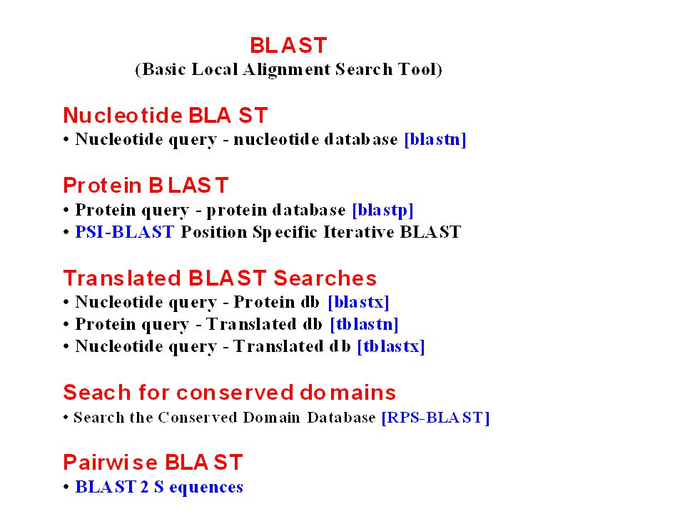
21. Methods: Important to know how algorithms that allow sequence comparisons work, There are many comparisons methods, Among most used: BLAST FASTA Smith-Waterman algorithm dynamic programming method HMM (Hidden Markov Model)

22. Sequence Comparaisons V I T K L G T C V G SV I T K L G T C V G S V I S... T Q V G SV. S K. G T Q V. S Identity Similarity Homology

23. Comparison of 2 sequences Aims at finding the optimal alignment: the one that shows most similar regions and regions that are less similar. In describing sequence comparisons, three different terms are commonly used : Identity, Similarity and Homology.  Need for a score that evaluates: - matches - mismatches - gaps  and a method that evaluates the numerous possible alignments.

24. Identity Refers to the occurence of identical nucleotides or amino acids in the same position in aligned sequences ; Identity is objective and well defined; Identity can be quantified: Percent i.e the number of identical matches divided by the length of the aligned region.

25. Similarity Sequence similarity takes approximate matches into account, and is meaningful only when such substitutions are scored according to some measure of «difference» with conservative substitutions assigned more favorable scores than non-conservative ones (substitution matrices). Given a number of parameters (alphabet, scoring matrix, filtering procedure, etc...), the similarity of an aligned region is defined by a score calculated on that region; The score depends on the chosen parameters; Contrarily to homology : expression like significant or weak similarity are often used.

26. Homology Sequence homology underlies common ancestry and sequence conservation; Homology can be inferred, under suitable conditions from sequence similarity ; The main objective of sequence similarity searching studies aims at inferring homology between sequences; Homology is not a measure. It is an all or none relashionship (i.e homology exits or does not exist. Expressions like : significant or weak homology are meaningless!). Sequence similarity is a measure of the matching characters in an alignment, whereas homology is a statement of common evolutionary origin.

27. Local Alignment Global Alignment

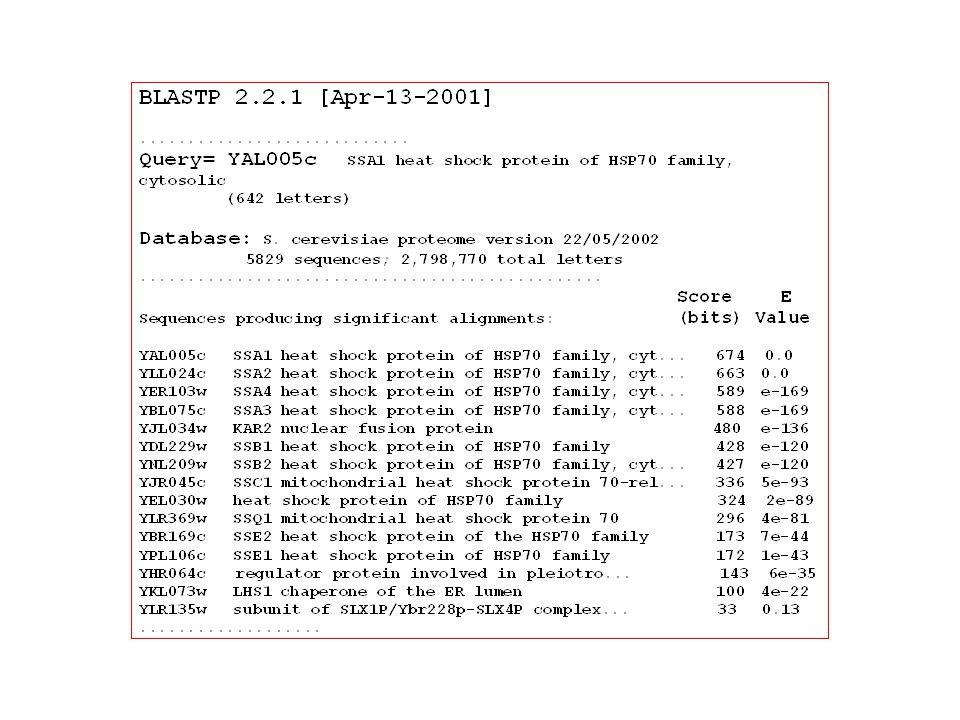
28. Compare one query sequence to a BLAST formatted database

29. Amino acid scoring schemes (substitution matrices) All algorithms comparing protein sequences rely on some schemes to score the equivalence of each of the 210 possible pairs of amino acids. As a result : what a local alignment program produces depends strongly upon the scores it uses. implicitly a scheme may represent a particular theory of evolution, choice of a matrix can strongly influence the outcome of an analysis. The scores in the matrix are integer values which assign a positive score to identical or similar character pairs, and a negative value to dissimilar character pairs. S ij = (ln(q ij /p i p j ))/ u ; q ij are target frequencies for aligned pairs of amino acids, the p i and p j are background frequencies, and u is a statistical parameter.

30. Examples of substitution matrices # PAM250 substitution matrix, scale = ln(2)/3 = 0.231049 # Expected score = -0.844, Entropy = 0.354 bits # Lowest score = -8, Highest score = 17 A R N D C Q E G H I L K M F P S T W Y V B Z X * A 2 -2 0 0 -2 0 0 1 -1 -1 -2 -1 -1 -3 1 1 1 -6 -3 0 0 0 0 -8 R -2 6 0 -1 -4 1 -1 -3 2 -2 -3 3 0 -4 0 0 -1 2 -4 -2 -1 0 -1 -8 N 0 0 2 2 -4 1 1 0 2 -2 -3 1 -2 -3 0 1 0 -4 -2 -2 2 1 0 -8 D 0 -1 2 4 -5 2 3 1 1 -2 -4 0 -3 -6 -1 0 0 -7 -4 -2 3 3 -1 -8 C -2 -4 -4 -5 12 -5 -5 -3 -3 -2 -6 -5 -5 -4 -3 0 -2 -8 0 -2 -4 -5 -3 -8 Q 0 1 1 2 -5 4 2 -1 3 -2 -2 1 -1 -5 0 -1 -1 -5 -4 -2 1 3 -1 -8 E 0 -1 1 3 -5 2 4 0 1 -2 -3 0 -2 -5 -1 0 0 -7 -4 -2 3 3 -1 -8 G 1 -3 0 1 -3 -1 0 5 -2 -3 -4 -2 -3 -5 0 1 0 -7 -5 -1 0 0 -1 -8 H -1 2 2 1 -3 3 1 -2 6 -2 -2 0 -2 -2 0 -1 -1 -3 0 -2 1 2 -1 -8 I -1 -2 -2 -2 -2 -2 -2 -3 -2 5 2 -2 2 1 -2 -1 0 -5 -1 4 -2 -2 -1 -8 L -2 -3 -3 -4 -6 -2 -3 -4 -2 2 6 -3 4 2 -3 -3 -2 -2 -1 2 -3 -3 -1 -8 K -1 3 1 0 -5 1 0 -2 0 -2 -3 5 0 -5 -1 0 0 -3 -4 -2 1 0 -1 -8 M -1 0 -2 -3 -5 -1 -2 -3 -2 2 4 0 6 0 -2 -2 -1 -4 -2 2 -2 -2 -1 -8 F -3 -4 -3 -6 -4 -5 -5 -5 -2 1 2 -5 0 9 -5 -3 -3 0 7 -1 -4 -5 -2 -8 P 1 0 0 -1 -3 0 -1 0 0 -2 -3 -1 -2 -5 6 1 0 -6 -5 -1 -1 0 -1 -8 S 1 0 1 0 0 -1 0 1 -1 -1 -3 0 -2 -3 1 2 1 -2 -3 -1 0 0 0 -8 T 1 -1 0 0 -2 -1 0 0 -1 0 -2 0 -1 -3 0 1 3 -5 -3 0 0 -1 0 -8 W -6 2 -4 -7 -8 -5 -7 -7 -3 -5 -2 -3 -4 0 -6 -2 -5 17 0 -6 -5 -6 -4 -8 Y -3 -4 -2 -4 0 -4 -4 -5 0 -1 -1 -4 -2 7 -5 -3 -3 0 10 -2 -3 -4 -2 -8 V 0 -2 -2 -2 -2 -2 -2 -1 -2 4 2 -2 2 -1 -1 -1 0 -6 -2 4 -2 -2 -1 -8 B 0 -1 2 3 -4 1 3 0 1 -2 -3 1 -2 -4 -1 0 0 -5 -3 -2 3 2 -1 -8 Z 0 0 1 3 -5 3 3 0 2 -2 -3 0 -2 -5 0 0 -1 -6 -4 -2 2 3 -1 -8 X 0 -1 0 -1 -3 -1 -1 -1 -1 -1 -1 -1 -1 -2 -1 0 0 -4 -2 -1 -1 -1 -1 -8 * -8 -8 -8 -8 -8 -8 -8 -8 -8 -8 -8 -8 -8 -8 -8 -8 -8 -8 -8 -8 -8 -8 -8 1

31. BLOSUM62 Clustered Scoring Matrix in 1/2 Bit Units # Cluster Percentage: >= 62 # Lowest score = -4, Highest score = 11 A R N D C Q E G H I L K M F P S T W Y V B Z X * A 4 -1 -2 -2 0 -1 -1 0 -2 -1 -1 -1 -1 -2 -1 1 0 -3 -2 0 -2 -1 0 -4 R -1 5 0 -2 -3 1 0 -2 0 -3 -2 2 -1 -3 -2 -1 -1 -3 -2 -3 -1 0 -1 -4 N -2 0 6 1 -3 0 0 0 1 -3 -3 0 -2 -3 -2 1 0 -4 -2 -3 3 0 -1 -4 D -2 -2 1 6 -3 0 2 -1 -1 -3 -4 -1 -3 -3 -1 0 -1 -4 -3 -3 4 1 -1 -4 C 0 -3 -3 -3 9 -3 -4 -3 -3 -1 -1 -3 -1 -2 -3 -1 -1 -2 -2 -1 -3 -3 -2 -4 Q -1 1 0 0 -3 5 2 -2 0 -3 -2 1 0 -3 -1 0 -1 -2 -1 -2 0 3 -1 -4 E -1 0 0 2 -4 2 5 -2 0 -3 -3 1 -2 -3 -1 0 -1 -3 -2 -2 1 4 -1 -4 G 0 -2 0 -1 -3 -2 -2 6 -2 -4 -4 -2 -3 -3 -2 0 -2 -2 -3 -3 -1 -2 -1 -4 H -2 0 1 -1 -3 0 0 -2 8 -3 -3 -1 -2 -1 -2 -1 -2 -2 2 -3 0 0 -1 -4 I -1 -3 -3 -3 -1 -3 -3 -4 -3 4 2 -3 1 0 -3 -2 -1 -3 -1 3 -3 -3 -1 -4 L -1 -2 -3 -4 -1 -2 -3 -4 -3 2 4 -2 2 0 -3 -2 -1 -2 -1 1 -4 -3 -1 -4 K -1 2 0 -1 -3 1 1 -2 -1 -3 -2 5 -1 -3 -1 0 -1 -3 -2 -2 0 1 -1 -4 M -1 -1 -2 -3 -1 0 -2 -3 -2 1 2 -1 5 0 -2 -1 -1 -1 -1 1 -3 -1 -1 -4 F -2 -3 -3 -3 -2 -3 -3 -3 -1 0 0 -3 0 6 -4 -2 -2 1 3 -1 -3 -3 -1 -4 P -1 -2 -2 -1 -3 -1 -1 -2 -2 -3 -3 -1 -2 -4 7 -1 -1 -4 -3 -2 -2 -1 -2 -4 S 1 -1 1 0 -1 0 0 0 -1 -2 -2 0 -1 -2 -1 4 1 -3 -2 -2 0 0 0 -4 T 0 -1 0 -1 -1 -1 -1 -2 -2 -1 -1 -1 -1 -2 -1 1 5 -2 -2 0 -1 -1 0 -4 W -3 -3 -4 -4 -2 -2 -3 -2 -2 -3 -2 -3 -1 1 -4 -3 -2 11 2 -3 -4 -3 -2 -4 Y -2 -2 -2 -3 -2 -1 -2 -3 2 -1 -1 -2 -1 3 -3 -2 -2 2 7 -1 -3 -2 -1 -4 V 0 -3 -3 -3 -1 -2 -2 -3 -3 3 1 -2 1 -1 -2 -2 0 -3 -1 4 -3 -2 -1 -4 B -2 -1 3 4 -3 0 1 -1 0 -3 -4 0 -3 -3 -2 0 -1 -4 -3 -3 4 1 -1 -4 Z -1 0 0 1 -3 3 4 -2 0 -3 -3 1 -1 -3 -1 0 -1 -3 -2 -2 1 4 -1 -4 X 0 -1 -1 -1 -2 -1 -1 -1 -1 -1 -1 -1 -1 -1 -2 0 0 -2 -1 -1 -1 -1 -1 -4 * -4 -4 -4 -4 -4 -4 -4 -4 -4 -4 -4 -4 -4 -4 -4 -4 -4 -4 -4 -4 -4 -4 -4 1

32. PAM matrices (Dayhoff et al. (1978)) PAM stands for “point accepted mutation”. 1 PAM corresponds to 1 amino acid change per 100 residues, 1 PAM ~1% divergence, Extrapolate to predict patterns at longer distances. Assumptions : replacements are independent of surrounding residues, sequences being compared are of average composition, all sites are equally mutable, Source of error : small, globular proteins were used to derive PAM matrices (departure from average composition) errors in PAM1 are magnified up to PAM250,.... does not account for conserved blocks or motifs. Strategy : PAM40short alignments, highly similar PAM120average similarity PAM250longer, weaker local alignments.

33. BLOSUM matrices (Henikoff, S., and Henikoff, J., G. (1992)) BlosumX denotes a matrix obtained from alignments of clustered sequence segments with more than X% identity. Examples : - Blosum62 is obtained from clustered sequences with identity greater than 62%. - Blosum80 is obtained from clustered sequences with identity greater than 80%. Which substitution matrix to choose? Blosum80Blosum62Blosum45 PAM10PAM120PAM250 Less divergent More divergent

35. Position Specific Scoring Matrix (PSSM) - Conserved motifs are identified and amino acid profile matrix for each motif is calculated. -This matrix (n x 20 aa ) is representative of the relative amino acid probabilities at specific positions and is characteristic of a protein family. -Such matrices are used by the profile database searching programs (including PSI-BLAST and HMM based programs).

36. Example of a PSSM matrices determined (PSI-BLAST program): A R N D C Q E G H I L K M F P S T W Y V 1 M -1 -1 -2 -3 -1 0 -2 -3 -2 1 2 -1 5 0 -2 -1 -1 -1 -1 1 2 S 1 -1 1 0 -1 0 0 0 -1 -2 -2 0 -1 -2 -1 4 1 -3 -2 -2 3 S 1 -1 1 0 -1 0 0 0 -1 -2 -2 0 -1 -2 -1 4 1 -3 -2 -2 4 S 1 -1 1 0 -1 0 0 0 -1 -2 -2 0 -1 -2 -1 4 1 -3 -2 -2 5 S 1 -1 1 0 -1 0 0 0 -1 -2 -2 0 -1 -2 -1 4 1 -3 -2 -2 6 G 0 -2 0 -1 -3 -2 -2 6 -2 -4 -4 -2 -3 -3 -2 0 -2 -2 -3 -3 7 L -1 -2 -3 -4 -1 -2 -3 -4 -3 2 4 -2 2 0 -3 -2 -1 -2 -1 1 8 K -1 2 0 -1 -3 1 1 -2 -1 -3 -2 5 -1 -3 -1 0 -1 -3 -2 -2 9 Q -1 1 0 0 -3 5 2 -2 0 -3 -2 1 0 -3 -1 0 -1 -2 -1 -2 10 Q -1 1 0 0 -3 5 2 -2 0 -3 -2 1 0 -3 -1 0 -1 -2 -1 -2 11 G 0 -2 0 -1 -2 -2 -2 6 -2 -4 -4 -2 -3 -3 -2 0 -2 -2 -3 -3 12 L -1 -2 -3 -4 -1 -2 -3 -4 -3 2 4 -2 2 0 -3 -2 -1 -2 -1 1 13 A 4 -1 -2 -2 0 -1 -1 0 -2 -1 -1 -1 -1 -2 -1 1 0 -3 -2 0 14 Q -1 1 0 0 -3 5 2 -2 0 -3 -2 1 0 -3 -1 0 -1 -2 -1 -2 15 K -1 2 0 -1 -3 1 1 -2 -1 -3 -2 5 -1 -3 -1 0 -1 -3 -2 -2 16 K -1 2 0 -1 -3 1 1 -2 -1 -3 -2 5 -1 -3 -1 0 -1 -3 -2 -2 17 K -1 2 0 -1 -3 1 1 -2 -1 -3 -2 5 -1 -3 -1 0 -1 -3 -2 -2 18 F -2 -3 -3 -3 -2 -3 -3 -3 -1 0 0 -3 0 6 -4 -2 -2 1 3 -1 19 Q -1 1 0 0 -3 5 3 -2 0 -3 -2 1 0 -3 -1 0 -1 -2 -1 -2 20 L -1 -2 -3 -4 -1 -2 -3 -4 -3 2 4 -2 2 0 -3 -2 -1 -2 -1 1 21 E -1 0 0 2 -4 2 5 -2 0 -3 -3 1 -2 -3 -1 0 -1 -3 -2 -2 22 F -2 -3 -3 -3 -2 -3 -3 -3 -1 0 0 -3 0 6 -4 -2 -2 1 3 -1 23 D -2 -2 1 6 -3 0 2 -1 -1 -3 -4 -1 -3 -3 -1 0 -1 -4 -3 -3..................................................................... 573 I -1 -3 -3 -3 -1 -3 -3 -4 -3 4 2 -3 1 0 -3 -2 -1 -3 -1 3 574 P -1 -2 -2 -1 -3 -1 -1 -2 -2 -3 -3 -1 -2 -4 7 -1 -1 -4 -3 -2 575 L -1 -2 -3 -4 -1 -2 -3 -4 -3 2 4 -2 2 0 -3 -2 -1 -2 -1 1

37. (2) Compare the word list to the database and identify exact matches. Blast algorithm: (3)For each word match, extend alignment in both directions to (1) Query sequence: list of high scoring words of length w. Query Sequence of length L Maximum of L-w+1 words; w=3,11..... List the words that score at least T using a substitution matrix (Bosum62 or PAM250,...)..... DB sequences Extract matches of words from word list. Maximal Segment Pairs (MSPs): HSPs find alignments with scores > S

38. E-values: Statistics of HSP scores are characterized by two parameters, K and. The expected number of HSPs with score at least S is given by: E = Kmne - S (Karlin & Altschul,1990). m and n are sequence lengths. E is the E-value for the score S. Bit scores: S ’ = ( S – lnK)/ln2 The E-value corresponding to a given bit score is : E = mn2 -S’. (note mn). P-values: The probability of finding exactly a HSPs with score >= S is given by : P(a) = e -E.E a /a! (Poisson distribution), where E is the E-value of S given by the above equation. Finding zero HSP with score >=S is P(0) = e -E, so the probability of finding at least one such HSP is : P = 1 - e -E.

41. Large-scale proteome comparisons

42. The expected number of HSPs with score at least S is given by: E = Kmne - S. m and n are sequence and database lengths.

43. Systematic Analysis of Completely Sequenced Organisms In silico species specific comparisons; Degree of ancestral duplication and of ancestral conservation between pairs of species; Families of paralogs (Partition-MCL); Families of orthologs (Partition-MCL); Determination of the protein dictionary (orthologs); Determination of protein conservation profiles;

44. Homologs - Paralogs - Orthologs Homologs: A 1, B 1, A 2, B 2 Paralogs : A 1 vs B 1 and A 2 vs B 2 Orthologs: A 1 vs A 2 and B 1 vs B 2 S1S1 S2S2 ab Sequence analysis Species-1Species-2 Duplication Ancestor Evolution Speciation A1A1 A2A2 B1B1 B2B2 A B A B A

45. Time Duplication Speciation A B Duplication G G1 G2 B-G2 1 B-G2 2 A-G2A-G1B-G1 orthologs outparalogs inparalogsoutparalogs Orthologs - inparalogs - outparalogs Sequence similarities between out-paralogs should be larger than those between orthologs and in-paralogs; Orthology assignments are consistent among several genome pairs; Orthologues are present in syntenic order Kuzniar A, van Ham RC, Pongor S, Leunissen JA. (2008). The quest for orthologs: finding the corresponding gene across genomes.Trends Genet. 24(11):539-51. Review.

46. Altenhoff AM, Dessimoz C. (2009). Phylogenetic and functional assessment of orthologs inference projects and methods. PLoS Comput Biol. 5(1):e1000262. Kuzniar A, van Ham RC, Pongor S, Leunissen JA. (2008). The quest for orthologs: finding the corresponding gene across genomes.Trends Genet. 24(11):539-51. Review. Gabaldon T. (2008). Large-scale assignment of orthology: back to phylogenetics?Genome Biol. 9(10):235. Moreno-Hagelsoeb G, Latimer K. (2008). Choosing BLAST options for better detection of orthologs as reciprocal best hits. Bioinformatics. 3 :319-324. Chen F, Mackey AJ, Vermunt JK, Roos DS (2007). Assessing performance of orthology detection strategies applied to eukaryotic genomes. PLoS ONE. 2:e383. Goodstadt L, Ponting CP (2006). Phylogenetic reconstruction of orthology, paralogy, and conserved synteny for dog and human. PLoS Comput Biol. 2:e133.

47. Working Examples Comparing S. cerevisiae (SC) genome with C. elegans (CE) genome

48. SC vs SC

49. - Paralogs - multiple matches - Partitions/clustering

50. SC/CECE/SC Reciprocal Best Hits (RBH)

51. segmatchSCCE

52. Conclusion Large-scale analyses of Completely sequenced genomes allow a systematic vision of genes, genome organization and their macro as well their micro evolutions. Starting step for further evolutionary analyses that will be dealt with during this course.

53. Practical sessions (see text)