Download presentation
Presentation is loading. Please wait.

1
Building an LBM Model The following is a mixture of MATLAB and C. Care must be taken, because array indexing begins at 1 in MATLAB and at 0 in C.

2
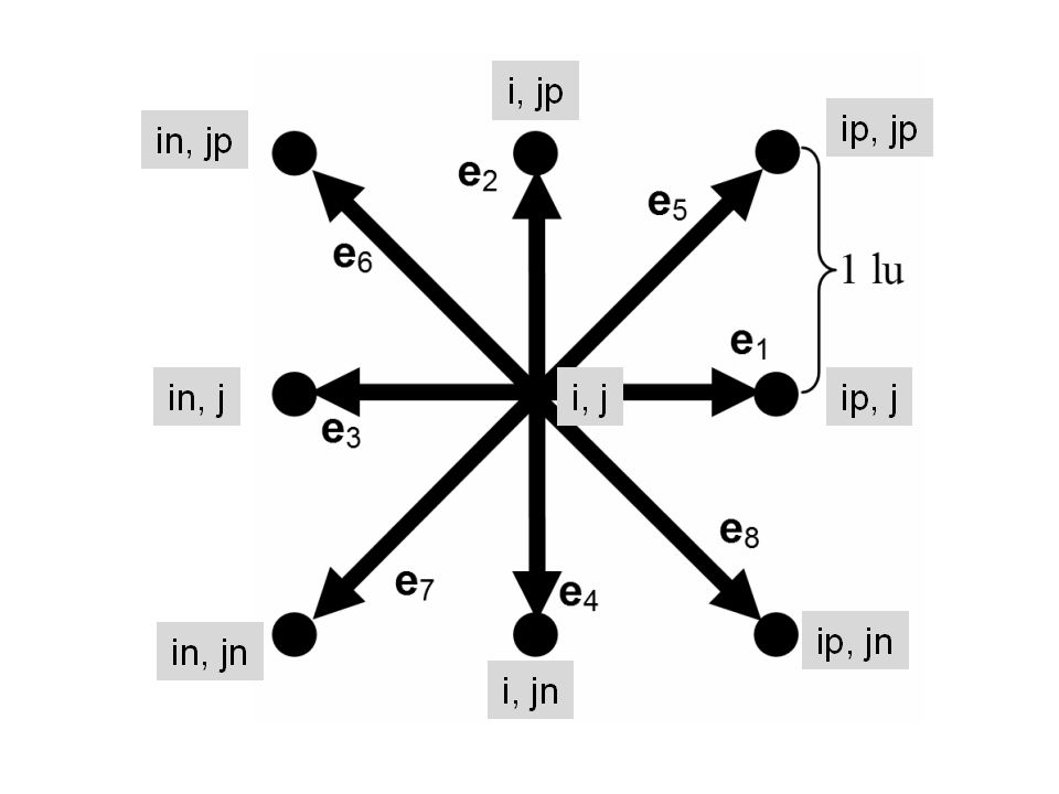
Define velocity vectors
1 2 3 4 5 6 7 8 D2Q9 e1 e2 e3 e4 e5 e6 e7 e8 %define es ex(0)= 0; ey(0)= 0 ex(1)= 1; ey(1)= 0 ex(2)= 0; ey(2)= 1 ex(3)=-1; ey(3)= 0 ex(4)= 0; ey(4)=-1 ex(5)= 1; ey(5)= 1 ex(6)=-1; ey(6)= 1 ex(7)=-1; ey(7)=-1 ex(8)= 1; ey(8)=-1 In MATLAB, can write ex(0+1)=0, ex(1+1)=1, etc.
= 0; ey(0)= 0. ex(1)= 1; ey(1)= 0. ex(2)= 0; ey(2)= 1. ex(3)=-1; ey(3)= 0. ex(4)= 0; ey(4)=-1. ex(5)= 1; ey(5)= 1. ex(6)=-1; ey(6)= 1. ex(7)=-1; ey(7)=-1. ex(8)= 1; ey(8)=-1. In MATLAB, can write ex(0+1)=0, ex(1+1)=1, etc.")
3
Problem definition LY=10 LX=20 tau = 1 g=0.00001 %set solid nodes
is_solid_node=zeros(LY,LX) for i=1:LX is_solid_node(1,i)=1 is_solid_node(LY,i)=1 end LY LX % if ~is_interior_solid_node(j,i)
 for i=1:LX. is_solid_node(1,i)=1. is_solid_node(LY,i)=1. end. LY. LX. % if ~is_interior_solid_node(j,i)")
4
Initialize density and fs (assuming zero velocity)
%define initial density and fs rho=ones(LY,LX); f(:,:,1) = (4./9. ).*rho; f(:,:,2) = (1./9. ).*rho; f(:,:,3) = (1./9. ).*rho; f(:,:,4) = (1./9. ).*rho; f(:,:,5) = (1./9. ).*rho; f(:,:,6) = (1./36.).*rho; f(:,:,7) = (1./36.).*rho; f(:,:,8) = (1./36.).*rho; f(:,:,9) = (1./36.).*rho;
; f(:,:,1) = (4./9. ).*rho; f(:,:,2) = (1./9. ).*rho; f(:,:,3) = (1./9. ).*rho; f(:,:,4) = (1./9. ).*rho; f(:,:,5) = (1./9. ).*rho; f(:,:,6) = (1./36.).*rho; f(:,:,7) = (1./36.).*rho; f(:,:,8) = (1./36.).*rho; f(:,:,9) = (1./36.).*rho;")
5
// Computing macroscopic density, rho, and velocity, u=(ux,uy).
for( j=0; j<LY; j++) { for( i=0; i<LX; i++) u_x[j][i] = 0.0; u_y[j][i] = 0.0; rho[j][i] = 0.0; if( !is_solid_node[j][i]) for( a=0; a<9; a++) rho[j][i] += f[j][i][a]; u_x[j][i] += ex[a]*f[j][i][a]; u_y[j][i] += ey[a]*f[j][i][a]; } u_x[j][i] /= rho[j][i]; u_y[j][i] /= rho[j][i];
 { for( i=0; i<LX; i++) u_x[j][i] = 0.0; u_y[j][i] = 0.0; rho[j][i] = 0.0; if( !is_solid_node[j][i]) for( a=0; a<9; a++) rho[j][i] += f[j][i][a]; u_x[j][i] += ex[a]*f[j][i][a]; u_y[j][i] += ey[a]*f[j][i][a]; } u_x[j][i] /= rho[j][i]; u_y[j][i] /= rho[j][i];")
7
Periodic Boundaries On boundary, ‘neighboring’ point is on opposite boundary ip = ( i<LX-1)?( i+1):( 0 ); in = ( i>0 )?( i-1):( LX-1); jp = ( j<LY-1)?( j+1):( 0 ); jn = ( j>0 )?( j-1):( LY-1); where LHS = (COND)?(TRUE_RHS):(FALSE_RHS); means if( COND) { LHS=TRUE_RHS;} else{ LHS=FALSE_RHS;}
 ( i-1):( LX-1); jp = ( j<LY-1) ( j+1):( 0 ); jn = ( j>0 ) ( j-1):( LY-1); where. LHS = (COND) (TRUE_RHS):(FALSE_RHS); means. if( COND) { LHS=TRUE_RHS;} else{ LHS=FALSE_RHS;}")
8
// Compute the equilibrium distribution function, feq.
for( j=0; j<LY; j++) { for( i=0; i<LX; i++) if( !is_solid_node[j][i]) rt0 = (4./9. )*rhoij; rt1 = (1./9. )*rhoij; rt2 = (1./36.)*rhoij; ueqxij = uxij; //Can add forcing here; see MATLAB code ueqyij = uyij; uxsq = ueqxij * ueqxij; uysq = ueqyij * ueqyij; uxuy5 = ueqxij + ueqyij; uxuy6 = -ueqxij + ueqyij; uxuy7 = -ueqxij + -ueqyij; uxuy8 = ueqxij + -ueqyij; usq = uxsq + uysq;
 { for( i=0; i<LX; i++) if( !is_solid_node[j][i]) rt0 = (4./9. )*rhoij; rt1 = (1./9. )*rhoij; rt2 = (1./36.)*rhoij; ueqxij = uxij; //Can add forcing here; see MATLAB code. ueqyij = uyij; uxsq = ueqxij * ueqxij; uysq = ueqyij * ueqyij; uxuy5 = ueqxij + ueqyij; uxuy6 = -ueqxij + ueqyij; uxuy7 = -ueqxij + -ueqyij; uxuy8 = ueqxij + -ueqyij; usq = uxsq + uysq;")
9
feqij[0] = rt0*( 1. - f3*usq);
feqij[1] = rt1*( 1. + f1*ueqxij + f2*uxsq f3*usq); feqij[2] = rt1*( 1. + f1*ueqyij + f2*uysq f3*usq); feqij[3] = rt1*( 1. - f1*ueqxij + f2*uxsq f3*usq); feqij[4] = rt1*( 1. - f1*ueqyij + f2*uysq f3*usq); feqij[5] = rt2*( 1. + f1*uxuy5 + f2*uxuy5*uxuy5 - f3*usq); feqij[6] = rt2*( 1. + f1*uxuy6 + f2*uxuy6*uxuy6 - f3*usq); feqij[7] = rt2*( 1. + f1*uxuy7 + f2*uxuy7*uxuy7 - f3*usq); feqij[8] = rt2*( 1. + f1*uxuy8 + f2*uxuy8*uxuy8 - f3*usq); }
![feqij[0] = rt0*( 1. - f3*usq);](http://slideplayer.com/slide/3359127/12/images/9/feqij%5B0%5D+%3D+rt0%2A%28+1.+-+f3%2Ausq%29%3B.jpg "feqij[1] = rt1*( 1. + f1*ueqxij + f2*uxsq - f3*usq); feqij[2] = rt1*( 1. + f1*ueqyij + f2*uysq - f3*usq); feqij[3] = rt1*( 1. - f1*ueqxij + f2*uxsq - f3*usq); feqij[4] = rt1*( 1. - f1*ueqyij + f2*uysq - f3*usq); feqij[5] = rt2*( 1. + f1*uxuy5 + f2*uxuy5*uxuy5 - f3*usq); feqij[6] = rt2*( 1. + f1*uxuy6 + f2*uxuy6*uxuy6 - f3*usq); feqij[7] = rt2*( 1. + f1*uxuy7 + f2*uxuy7*uxuy7 - f3*usq); feqij[8] = rt2*( 1. + f1*uxuy8 + f2*uxuy8*uxuy8 - f3*usq); }")
10
Collide // Collision step. for( j=0; j<LY; j++)
for( i=0; i<LX; i++) if( !is_solid_node[j][i]) for( a=0; a<9; a++) { fij[a] = fij[a] + ( fij[a] - feqij[a])/tau; }
 if( !is_solid_node[j][i]) for( a=0; a<9; a++) { fij[a] = fij[a] + ( fij[a] - feqij[a])/tau; }")
11
Bounceback Boundaries
Bounceback boundaries are particularly simple Played a major role in making LBM popular among modelers interested in simulating fluids in domains characterized by complex geometries such as those found in porous media Their beauty is that one simply needs to designate a particular node as a solid obstacle and no special programming treatment is required

12
Two type of solids:

13
Bounceback Boundaries

14
Collision (solid nodes): Bounceback
// Standard bounceback. temp = fij[1]; fij[1] = fij[3]; fij[3] = temp; temp = fij[2]; fij[2] = fij[4]; fij[4] = temp; temp = fij[5]; fij[5] = fij[7]; fij[7] = temp; temp = fij[6]; fij[6] = fij[8]; fij[8] = temp;

15
// Streaming step. for( j=0; j<LY; j++) { jn = (j>0 )?(j-1):(LY-1) jp = (j<LY-1)?(j+1):(0 ) for( i=0; i<LX; i++) if( !is_interior_solid_node[j][i]) in = (i>0 )?(i-1):(LX-1) ip = (i<LX-1)?(i+1):(0 ) ftemp[j ][i ][0] = f[j][i][0]; ftemp[j ][ip][1] = f[j][i][1]; ftemp[jp][i ][2] = f[j][i][2]; ftemp[j ][in][3] = f[j][i][3]; ftemp[jn][i ][4] = f[j][i][4]; ftemp[jp][ip][5] = f[j][i][5]; ftemp[jp][in][6] = f[j][i][6]; ftemp[jn][in][7] = f[j][i][7]; ftemp[jn][ip][8] = f[j][i][8]; }
 in = (i>0 ) (i-1):(LX-1) ip = (i<LX-1) (i+1):(0 ) ftemp[j ][i ][0] = f[j][i][0]; ftemp[j ][ip][1] = f[j][i][1]; ftemp[jp][i ][2] = f[j][i][2]; ftemp[j ][in][3] = f[j][i][3]; ftemp[jn][i ][4] = f[j][i][4]; ftemp[jp][ip][5] = f[j][i][5]; ftemp[jp][in][6] = f[j][i][6]; ftemp[jn][in][7] = f[j][i][7]; ftemp[jn][ip][8] = f[j][i][8]; }")
16
Incorporating Forcing (gravity)
Gravitational acceleration is incorporated in a velocity term ueqxij = u_x(j,i)+tau*g; %add forcing
+tau*g; %add forcing.")
Similar presentations


![Vector: Data Layout Vector: x[n] P processors Assume n = r * p](/11/3276141/big_thumb.jpg "Vector: Data Layout Vector: x[n] P processors Assume n = r * p>")


 Compact notation using vector del, or nabla: Another notation: Partial derivative is.>")


