1. Coalescent Theory & Population Genetics applications Frantz Depaulis depaulis@ens.frdepaulis@ens.fr http://www.biologie.ens.fr/eceem/frantz_depaulis Pwd: M1ENSCOAL Laboratoire Ecologie et Evolution, CNRS-UMR 7625 Université Paris 6- ENS room 426

2. Outline Reminder Coalescence Mutations/models Perturbations, applications

3. Neutral theory of molecular evolution (Kimura 1969): the neutral model as a reference Mutations Occurrence Fate avantageous rarefixed deleteriousfrequenteliminated neutralfrequent drift until fixation or loss -reminder-

4. Wright Fisher Neutral model Assumptions Selective neutrality (N e s <<1) Demography - Isolated panmictic Population, - Constant size N - Poisson Distribution of offspring P (1) -reminder-

5. Effectif efficace : définition On définit la taille efficace (notée N e ) d’une population comme étant la taille d’une population « idéale » de Wright-Fisher où la dérive génétique aurait la même intensité (**) que dans la population (ou bien le modèle de population) qui nous intéresse ** même taux de dérive, même augmentation de consanguinité, même augmentation de variance de fréquences alléliques entre populations, etc. -reminder-

6. Relationships among 10 individuals over 15 generations GenerationsGenerations individuals # genes -Coalescence-

7. the same, but permuted GenerationsGenerations individuals # genes -Coalescence-

8. Descent and extinction of a lineage GenerationsGenerations individuals # genes -Coalescence-

9. Genealogy of 3 individuals: Regarder le processus de dérive en « remontant le temps » jusqu’à l’ancêtre commun d’un échantillon de gènes GenerationsGenerations individuals#genes -Coalescence-

10. Genealogy of a gene sample gene sample ancestral lineage coalescence= common ancestor Most recent common ancestor (MRCA) -Coalescence-

11. Kingman (1980, 1982)

12. -Coalescence-

15. Coalescent Tree ab cde f Most recent common ancestor of the sample (MRCA) sample of “genes” / of individuals Common ancestor (CA) neutral mutations T C C G C G A A -Coalescence-

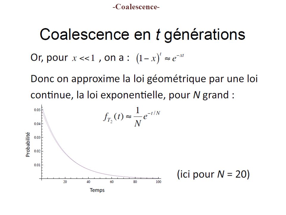
26. Coalescent times 2 genes p 2 =P( common ancestry in t -1)= 1/2N n genes p n =P ( common ancestry at t -1)= (n x (n -1)/2) x 1/2N P ( common ancestry t generations ago ) = (1-p) t -1 x p Geometric distribution (discrete generations) #p e (-pt ) Exponential distribution (continuous time) p small, t large t t-1 1/2N 1 2 3 4 5... 2N... -Coalescence- Diploïde (2n) => 2N genes

27. -Coalescence-

30. Effectif efficace de consanguinité Dans le modèle de Wright-Fisher, la probabilité de coalescence en une génération est égale à 1/N. On peut donc définir une taille efficace comme l’inverse de la probabilité de coalescence en une génération (Ewens, 1982). C’est une taille efficace de consanguinité, et qui est instantanée. Au contraire, une taille efficace asymptotique peut être définie, qui décrit le taux de coalescence de lignées de gènes dans un passé lointain (égale à 1/N dans le modèle de Wright-Fisher) Cette taille efficace asymptotique (de consanguinité, de coalescence) est équivalente à la taille efficace de valeur propre, qui repose sur une description complète des fréquences alléliques dans une population (la valeur propre de la matrice qui décrit les changements de fréquence détermine l’approche de l’état d’équilibre) -Coalescence-

31. 1°) Ages of the nodes Constructing coalescents, cdefba t3t3 p =1/2N Exp( p ) t1t1 t2t2 t4t4 t5:t5: additional assumption: n << N -Coalescence-

32. gene sample Topology of the tree 2°) abcdef MRCA common ancestor (CA) t1t1 t2t2 t3t3 t4t4 t5:t5: Constructing- deconstructing coalescents -Coalescence- http://www.coalescent.dk/ Hudson’s animator:

33. Mutations and associated models -Mutations-

35. AA A A neutral mutations G T C C G C A 3°) uniform distribution of mutations gene sample Topology of the tree 2°) T C G A C G C T neutral distribution of sequence polymorphism abcdef MRCA common ancestor (CA) t1t1 t2t2 t3t3 t4t4 t5:t5: 100 000 times Constructing- deconstructing coalescents S : P ( T Tot x  )  =4N e µ -Mutations-

36. Mutational, sequence data: infinite site model (ISM) - No recombination - Independent mutations - Constant mutation rate µ Along the sequence Across time - Each mutation affects a new nucleotide site Infinite(ly many) site model: sequences, SNP’s -Mutations-

37. GCCCGCGAATCCATT GCGTGCGATCCGATT GCGTACAATCCCGTC GTGTACAATCTCGAC GCGTGGAATCCCGTT CCGCGCGGTCCCATT f 121531416121423 T C T AC T G A T G C Alignment of polymorphic sites: G T G n =7 S =15 -Mutations-

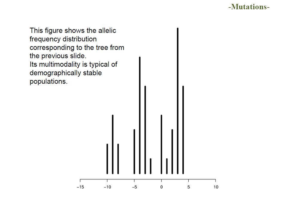
38. Frequency spectrum of mutations f i : Number of polymorphic sites Number of occurrences in a sample Neutral predictions -Mutations- Watterson’s (1975) estimator  =4N e  * *: Tajima (1983)

39. f 121531416621423 f 121531416121423 GCCCGCGAATCCATT GCGTGCGATCCGATT GCGTACAATCCCGTC GTGTACAATCTCGAC GCGTGGAATCCCGTT CCGCGCGGTCCCATT GCCCGCGAATCCATT GCGTGCGATCCGATT GCGTACAATCCCGTC GTGTACAATCTCGAC GCGTGGAATCCCGTT CCGCGCGGTCCCATT CTCT → TCTC → T C T AC T G A T G C Alignment of polymorphic sites: non oriented mutations G T G n =7 S =15 -Mutations-

40. Frequency spectrum of mutations f i : number of occurrences in a sample Number of polymorphic sites -Mutations-

41. GCCCGCGAATCCATT GCGTGCGATCCGATT GCGTACAATCCCGTC GTGTACAATCTCGAC GCGTGGAATCCCGTT CCGCGCGGTCCCATT f 121531416121423 CTCT → Alignment of polymorphic sites: orienting mutations with an outgroup f 121531416621423 TCTC → GCCCGCGAATCCATT GCGTGCGATCCGATT GCGTACAATCCCGTC GTGTACAATCTCGAC GCGTGGAATCCCGTT CCGCGCGGTCCCATT T C o.g.GCGCGCGAACCCATT C -Mutations-

42. Infinite(ly many) allele model: allozymes, one site (locus) (microsatellites) Each mutation gives rise to a new type/allele on a locus T A C C G C G T G GG CC A A A T C C A T -Mutations-

43. The “stepwise mutation” model (SMM) is appropriate for microsatellites. When a mutation occurs, the new mutation length depends on the existing length. In the simplest case of the “single” SMM, illustrated in the next slide, the new length = old length +/- 1. Stepwise mutation model -Mutations-

44. Microsatellites GAGGCGTAGTAGTAGTAGTAGTAGTAGGCTCTA GAGGCGTAGTAGTAGTAGTAGTAGGCTCTA or GAGGCGTAGTAGTAGTAGTAGTAGTAGTAGGCTCTA Microsatellites mutate very fast (~1 change every 500 generations) Mutation events usually involve a gain or a loss of a single repeat unit -Mutations-

47. Recombination « simple » case: 2 haplotypes with 2 locus One possible Genealogy outcome Recombination Coalescence MRCA1 MRCA2 Past -Perturbations-

48. Ancestral Recombination Graph : example coalescence rate : n(n-1)/2 recombination rate : R n Recombination Coalescence n =2 n =3 n =2 n =2 ? MRCA Time Past -Perturbations-

49. Recombination Histories: Non-ancestral bridges -Perturbations-

50. systematic effects  Genealogy  Demographic  Selective Extinction-recolonisation, severe bottlenecks, population expansion severe hitchhiking Migration, population structure, moderate bottlenecks balanced polymorphism, moderate hitchhiking -Perturbations-

51. The neutral model, application = inference  Applications Molecular phylogeography Molecular ecology: Selective effects - balancing selection - directional selection, hitchhiking Demographic effects - Dispersion - bottlenecks/expansion - Distribution of the number of offsprings  Tool= the coalescent -Coalescence-

52. -Perturbations- Demographic change

53. -Perturbations-

55. (a) Constant population size (simulation case 3) (b) Population expansion,  = 3 (simulation case 2) KK -Perturbations-

56. Coalescent and bottlenecks t N P t = 1/2N t -Perturbations-

57. Time Coalescence Migration Coalescence Pop 1 Pop 2 -Perturbations- Population structure Coalescence 1/m Migration

58. -Perturbations-

60. ______T_____*___C__ _G______A________G_ ACGTTTATGCAACGTCGAC 1°) an advantageous mutation appears 2°) Selection _G_______________G_ _________________G_ ______T____________ ______T_____*___C__ ACGTTTATGCAACGTCGAC ______T_____*___C__ 3°) Hitch-hiking effect: the advantageous mutation is fixed and variability is swept ACGTTTATGCAACGTCGAC Reference chromosomes population of chromosomes neutral mutations _G_______________G_ _________________G_ ______T____________ ______T_________C__ Selection: Hitch-hiking without recombination -Perturbations-

61. A Hitch-hiking without recombination: genealogy apparition of an advantageous mutation Few mutations at low frequency common ancestor T ****** T * A After hitch-hiking Neutral distribution of mutations in the sample T A C C G C G C C G AA C T T G A A neutral coalescent -Perturbations-

62. The effect of a selective sweep on the shape of the coalescent tree -Perturbations-

63. _G______A________G_ ACGTTTATGCAACGTCGAC 1°) an advantageous mutation appears 2°) Selection _G_______________G_ _________________G_ ______T____________ ______T_____*___C__ ACGTTTATGCAACGTCGAC _G______A___*___C__ ______T_____*___C__ 3°) Hitchhiking effect: several haplotypes remain ACGTTTATGCAACGTCGAC Reference chromosomes population of chromosomes neutral mutations _G_______________G_ _________________G_ ______T____________ ______T_________C__ hitchhiking with recombination _G______A___*___C__ -Perturbations-

64. hitchhiking with recombination: genealogy apparition of an advantageous mutation substantial number of high frequency mutations common ancestor ****** * After hitchhiking T A C C G C G C C G AA C T T G A A Neutral coalescent C G C G C G * recombination GGGG G Neutral distribution of mutations in the sample -Perturbations-

65. Frequency spectrum of mutations f i : Number of polymorphic sites Number of occurrence s in a sample Neutral predictionsSelective predictions -Perturbations-

68. /Background selection Charlesworth et al. 1993

69. Alternative hypotheses, overview S 15992 Neutral Moderate bottleneck /population structure Balanced selection hitchhiking with recombination Severe bottleneck, population expansion /local hitchhiking number of mutations perturbation -Perturbations- frequency class in excess intermediatehighlowNone

70. Gene genealogies / Coalescent theory Based on the standard Wright-Fisher neutral model Genealogical trees – backward – Intuitive – Economic * Sampling theory * Only generations where « events » occurred are considered -Coalescence- The coalescent= a simple and efficient framework to build make inference about selective and demographic history of populations

71. Acknowledgements –R. Vitalis –V. Castric –L. Chikki –S. Billiard –M. Schierup Oxf. Surv Evol Biol 1990. 7:1-44 http://home.uchicago.edu/~rhudson1/popgen356/OxfordSurveysEvolBiol7_1-44.pdf

73. Frequency spectrum of mutations f i : Number of polymorphic sites  =4N e  H=-HH=-H = 0= 0= 0= 0 = 0.05 = -3.01 * Number of occurrence s in a sample (Fay and Wu Genetics 2000) -Misorientation-

74. f 121531416621423 f 121531416121423 C C T GCCCGCGAATCCATT GCGTGCGATCCGATT GCGTACAATCCCGTC GTGTACAATCTCGAC GCGTGGAATCCCGTT CCGCGCGGTCCCATT GCCCGCGAATCCATT GCGTGCGATCCGATT GCGTACAATCCCGTC GTGTACAATCTCGAC GCGTGGAATCCCGTT CCGCGCGGTCCCATT o.g.GCGCGCGAACCCATTo.g.GCGCGCGAATCCATT TCTC → T T CTCT → T C pMpM Alignment of polymorphic sites: multiple hits and misorientation -Misorientation-

75. T A C C G C G C C G AA C TT G A A T A A C G T C C T C AA T T G A T C T A C C G C G C T G GG CC C G A A A A T Neutrality tests: simulations parameters ‡ : S =8 n =6 H = 2.13 H = -1.06... 10 000 simulations H {H { C C A T -tests- ‡ Hudson 1993 -3-201234 H density observed H : P = 0.03 * Distribution of simulated H