Download presentation
Presentation is loading. Please wait.

1
Regression analysis Relating two data matrices/tables to each other Purpose: prediction and interpretation Y-data X-data

2
Typical examples Spectroscopy: Predict chemistry from spectral measurements Product development: Relating sensory to chemistry data Marketing: Relating sensory data to consumer preferences

3
Topics covered Simple linear regression The selectivity problem: a reason why multivariate methods are needed The collinearity problem: a reason why data compression is needed The outlier problem: why and how to detect

4
Simple linear regression One y and one x. Use x to predict y. Use a linear model/equation and fit it by least squares

5
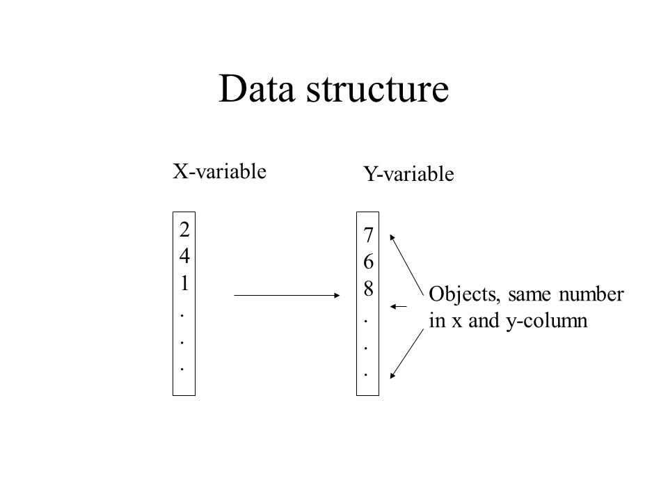
Data structure Y-variable X-variable Objects, same number in x and y-column 241...241... 768...768...
6
b0b0 b1b1 y=b 0 +b 1 x+e x y Least squares (LS) used for estimation of regression coefficients Simple linear regression
 used for estimation of regression coefficients Simple linear regression")
7
Model Data (X,Y) Regression analysis Future XPrediction Regression analysis Outliers? Pre-processing Interpretation

8
The selectivity problem A reason why multivariate methods are needed

9
Can be used for several Y’s also

10
Multiple linear regression Provides –predicted values –regression coefficients –diagnostics If there are many highly collinear variables –unstable regression equations –difficult to interpret coefficients: many and unstable

11
y=b 0 +b 1 x 1 +b 2 x 2 +e The two x’s have high correlation Leads to unstable equation/plane (in the direction with little variability) Collinearity, the problem of correlated X-variable Regression in this case is fitting a plane to the data (open circles)
 Collinearity, the problem of correlated X-variable Regression in this case is fitting a plane to the data (open circles)")
12
Possible solutions Select the most important wavelengths/variables (stepwise methods) Compress the variables to the most dominating dimensions (PCR, PLS) We will concentrate on the latter (can be combined)
 Compress the variables to the most dominating dimensions (PCR, PLS) We will concentrate on the latter (can be combined)")
13
Data compression We will first discuss the situation with one y-variable Focus on ideas and principles Provides regression equation (as above) and plots for interpretation
 and plots for interpretation")
14
Model for data compression methods X=TP T +E y=Tq+f T-scores, carrier of information from X to y P,q –loadings E,f – residuals (noise) Centred X and y
 Centred X and y")
15
Regression by data compression Regression on scores PC1 t-score y q titi PCA to compress data x1x1 x2x2 x3x3

16
x4 x1 x2 x3 x4 x2 x3 x1 x2 x4 x3 y y y t1 t2 MLR PCR PLS x1 t1 t2

17
PCR and PLS For each factor/component PCR –Maximize variance of linear combinations of X PLS –Maximize covariance between linear combinations of X and y Each factor is subtracted before the next is computed

18
Principal component regression (PCR) Uses principal components Solves the collinearity problem, stable solutions Provides plots for interpretation (scores and loadings) Well understood Outlier diagnostics Easy to modify But uses only X to determine components
 Uses principal components Solves the collinearity problem, stable solutions Provides plots for interpretation (scores and loadings) Well understood Outlier diagnostics Easy to modify But uses only X to determine components")
20
PLS-regression Easy to compute Stable solutions Provides scores and loadings Often less number of components than PCR Sometimes better predictions

21
PCR and PLS for several Y- variables PCR is computed for each Y. Each Y is regressed onto the principal components PLS: The algorithm is easily modified. Maximises linear combinations of X and Y. For both methods: Regression equations and plots

22
Validation is important Measure quality of the predictor Determine A – number of components Compare methods

23
Prediction testing Calibration Estimate coefficients Testing/validation Predict y, use the coefficients

24
Cross-validation Predict y, use the coefficients Calibrate, find y=f(x) estimate coefficients
 estimate coefficients")
25
Validation Compute Plot RMSEP versus component Choose the number of components with best RMSEP properties Compare for different methods

26
RMSEP NIR calibration of protein in wheat. 6 NIR wavelengths 12 calibration samples, 26 test samples MLR

27
Conceptual illustration of important phenomena Estimation error Model error

28
Prediction vs. cross-validation Prediction testing: Prediction ability of the predictor at hand. Requires much data. Cross-validation: Property of the method. Better for smaller data set.

29
Validation One should also plot measured versus predicted y-value Correlation can be computed, but can sometimes be misleading

30
Plot of measured and predicted protein NIR calibration Example, plot of y versus predicted y

31
Outlier detection Instrument error or noise Drift of signal (over time) Misprints Samples outside normal range (different population)
 Misprints Samples outside normal range (different population)")
32
Outlier detection Outliers can be detected because –Model for spectral data (X=TP T +E) –Model for relationship between X and y (y=Tq+f)
 –Model for relationship between X and y (y=Tq+f)")
33
Outlier detection tools Residuals –X and y-residuals –X-residuals as before, y-residual is difference between measured and predicted y Leverage –h i

Similar presentations


