1. An Introduction to the EM Algorithm Naala Brewer and Kehinde Salau

2. An Introduction to the EM Algorithm Outline History of the EM Algorithm Theory behind the EM Algorithm Biological Examples including derivations, coding in R, Matlab, C++ Graphs of iterations and convergence

3. Brief History of the EM Algorithm Method frequently referenced throughout field of statistics Term coined in 1977 paper by Arthur Dempster, Nan Laird, and Donald Rubin

4. Breakdown of the EM Task To compute MLEs of latent variables and unknown parameters in probabilistic models E-step: computes expectation of complete/unobserved data M-step: computes MLEs of unknown parameters Repeat!!

5. Generalization of the EM Algorithm X- Full sample (latent variable) ~ f(x; θ) Y - Observed sample (incomplete data) ~ f(y;θ) such that y(x) = y We define Q(θ;θ p ) = E[lnf(x;θ)|Y, θ p ] θ p+1 obtained by solving, = 0

6. Generalization (cont.) Iterations continue until |θ p+1 - θ p | or | Q(θ p+1 ;θ p ) - Q(θ p ;θ p ) | are sufficiently small Thus, optimal values for Q(θ;θ p ) and θ are obtained Likelihood nondecreasing with each iteration: Q(θ p+1 ;θ p ) ≥ Q(θ p ;θ p )

7. Example 1 - Ecological Example n - number of marked animals in 5 different regions, p - probability of survival Suppose that only the number of animals that survive in 3 of the 5 regions is known (we may not be able to see or capture all of the animals in x 1, x 2 ) X = (?, ?, 30, 25, 39) = (x 1, x 2, x 3, x 4, x 5 ) We estimate p using the EM Algorithm.

8. Binomial Distribution - Derivation

9. Binomial Derivation (cont.)

11. Binomial Distribution Graph of Convergence of Unknown Parameter, p k

12. Example 2 – Population of Animals Rao (1965, pp.368-369), Genetic Linkage Model Suppose 197 animals are distributed multinomially into four categories, y = (125, 18, 20, 34) = ( y 1, y 2, y 3, y 4 ) A genetic model for the population specifies cell probabilities (1/2+p /4, ¼ – p /4, ¼ – p/4, p/4) Represent y as incomplete data, y 1 =x 1 +x 2 (x 1, x 2 unknown), y 2 =x 3, y 3 =x 4, y 4 =x 5.

13. Multinomial Distribution-Derivation

14. Multinomial Derivation (cont.)

17. Multinomial Coding Example 2 – Population of Animals R Coding Matlab Coding C++ Coding

18. R Coding #initial vector of data y <- c(125, 18, 20, 34) #Initial value for unknown parameter pik <-.5 for(k in 1:10){ x2k <-y[1]*(.25*pik)/(.5 +.25*pik) pik <- (x2k + y[4])/(x2k + sum(y[2:4])) print(c(x2k,pik)) #Convergent values } Matlab Coding %initial vector of data y = [125, 18, 20, 34]; %Initial value for unknown parameter pik =.5; for k = 1:10 x2k = y(1)*(.25*pik)/(.5 +.25*pik) pik = (x2k + y(4))/(x2k + sum(y(2:4))) end %Convergent values [x2k,pik] Multinomial Coding

19. C++ Coding #include int main () { int x1, x2, x3, x4; float pik, x2k; std::cout << "enter vector of values, there should be four inputs\n"; std::cin >> x1 >> x2 >> x3 >> x4; std::cout << "enter value for pik\n"; std::cin >> pik; for (int counter = 0; counter < 10; counter++){ x2k = x1*((0.25)*pik)/((0.5) + (0.25)*pik); pik = (x2k + x4)/(x2k + x2 + x3 + x4); std::cout << "x2k is " << x2k << " and " << " pik is " << pik << std::endl; } return 0; } Matlab Coding %initial vector of data y = [125, 18, 20, 34]; %Initial value for unknown parameter pik =.5; for k = 1:10 x2k = y(1)*(.25*pik)/(.5 +.25*pik) pik = (x2k + y(4))/(x2k + sum(y(2:4))) end %Convergent values [x2k,pik] Multinomial Coding

20. Graphs of Convergence of Unknowns,p k and x 2 k Multinomial Distribution

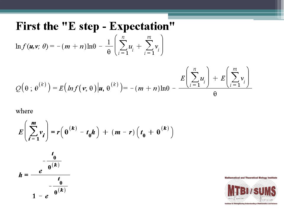
21. Example 3 -Failure Times Flury and Zoppè (2000) ▫Suppose the lifetime of bulbs follows an exponential distribution with mean θ ▫The failure times (u 1,...,u n ) are known for n light bulbs ▫In another experiment, m light bulbs (v 1,...,v m ) are tested; no individual recordings  The number of bulbs, r, that fail at time t 0 are recorded

22. Exponential Distribution - Derivation

24. Exponential Derivation (cont.)

25. Example 3 – Failure Times Graphs

26. Future Work More Elaborate Biological Examples Develop lognormal models with predictive capabilities for optimal interrupted HIV treatments (ref. H.T. Banks); i.e.Normal Mixture models Study of improved models Monte Carlo implementation of the E step Louis' Turbo EM

27. An Introduction to the EM Algorithm References [1] Dempster, A.P., Laird, N.M., Rubin, D.B. (1977). Maximum Likelihood from Incomplete Data via the EM Algorithm. Journal of the Royal Statistical Society. Series B (Methodological), Vol. 39, No. 1,, pp. 1-38 [2] Redner, R.A., Walker, H.F. (Apr., 1984). Mixture Densities, Maximum Likelihood and the EM Algorithm. SIAM Review, Vol. 26, No. 2., pp. 195-239. [3] Tanner, A.T. (1996). Tools for Statistical Inference. Springer- Verlag New York, Inc. Third Edition

28. Acknowledgements The MTBI/SUMS Summer Research Program is supported by:  The National Science Foundation (DMS-0502349)  The National Security Agency (DOD-H982300710096)  The Sloan Foundation  Arizona State University Our research particularly appreciates:  Dr. Randy Eubank  Dr. Carlos Castillo-Chavez