1. XPath Query Processing DBPL9 Tutorial, Sept. 8, 2003, Part 2 Georg Gottlob, TU Wien Christoph Koch, U. Edinburgh Based on joint work with R. Pichler

2. Contents Part 1 Xpath Basics Axis Evaluation Experiments with current systems Polynomial-time evaluation of Core Xpath Core XPath and datalog Polynomial-time evaluation of full Xpath Part 2 Context simplification and efficient evaluation of Xpath Parallel complexity of Xpath Automata-based techniques: –Xpath on Streaming XML –Expressive queries and automata. Further relevant work

3. Context Simplification and Efficient Evaluation of XPath

4. Time and space bound Bottom-up evaluation based on CVT: –Time O(|data| 5 * |query| 2 ), space O(|data| 4 * |query| 2 ). Space bound (n … number of nodes in input document.): Contexts are at most triples: at most n^3 contexts. Sizes of values: –Node sets: at most O(n) –Strings, numbers: at most O( |data|* |query|) – (iterated concatenation of strings, multiplication of numbers)  Each CVT is of size (|data| 4 * |query|). Time bound: most expensive computation is O(n^2) – Relational operation “=“ on node sets (e.g. a/b//c[d//e/f/g = h/i//j])

5. Alternative context representation Contexts represented as (“previous context node, “current context node”) rather than (“context node”, “position”, “size”). Need to recompute “position” and “size” on demand. Complexity lowered to time O(|data| 4 * |query| 2 ), space O(|data| 3 * |query| 2 ). //a/b[position() + 1 = size()] 1:a5:a 6:b7:b2:b3:b4:b 0:c child::b … { (1,2), (1,3), (1,4), (5,6), (5,7) } child::b[position()+1=size()] … { (1,3), (5,6) }

6. Context Simplification Technique 1.Only materialize relevant context. 2.Core Xpath evaluation algorithm for outermost and innermost paths //a/b/c//d[…]/e[…(a/b/c)]. 3.Treating “position” and “size” in a loop. Because of tree shape of query, loops never have to be nested. position() +1 = last() position() = count( )descendant::a /child::b[ ] (cn) (cn,cp, cs) - loop child::b[ ] Compute node set for which child::b[…] is true (cn,cp, cs) - loop

7. “Wadler Fragment” [Wadler, 1999]: Core Xpath + position(), last(), and arithmetics. Evaluation in quadratic time and linear space. For x in [[//a]] compute contexts (y,p,n) in x.[[b]] Compute Y = { y | (y,p,n) 2 x.[[b]] and p*2=n }. Similarly, compute Z = { z | z.[[ d[position()*3 = last()] ]] is true}. Compute X = { x | z 2 Z, x 2 z.[[ child::c ]] -1 } – in linear time. Result is { w | v \in X \cap Y, w \in v.[[descendant::e]] }. Linear Space Fragment //a/b[position() * 2 = last() and c/d[position()*3 = last()]]//e (cn) (cn,cp,cs) (cn) (cn,cp,cs)

8. Summary Full XPath Bottom-up algorithm based on CVT –Time O(|data| 5 * |query| 2 ), space O(|data| 4 * |query| 2 ). Top-down evaluation –Time O(|data| 4 * |query| 2 ), space O(|data| 3 * |query| 2 ). Context-reduction technique –Time O(|data| 4 * |query| 2 ), space O(|data| 2 * |query| 2 ). Wadler fragment –Time O(|data| 2 * |query| 2 ), space O(|data| * |query|). Core Xpath –Time and space O(|data| * |query|).

9. Parallel Complexity of XPath

10. Known: Xpath is in P w.r.t. combined complexity [G., K., and Pichler, VLDB 2002]. P-hardness => unlikely that there is an efficient parallel algorithm (conjecture: P > NC) Even quite restrictive fragments of Xpath are P-hard –Core Xpath using only child, parent, and descendant axes, no “branching” of tree patterns. –Proof by encoding circuits, somewhat involved! But: without negation, Core Xpath is in LOGCFL (< NC2, highly parallelizable!!)

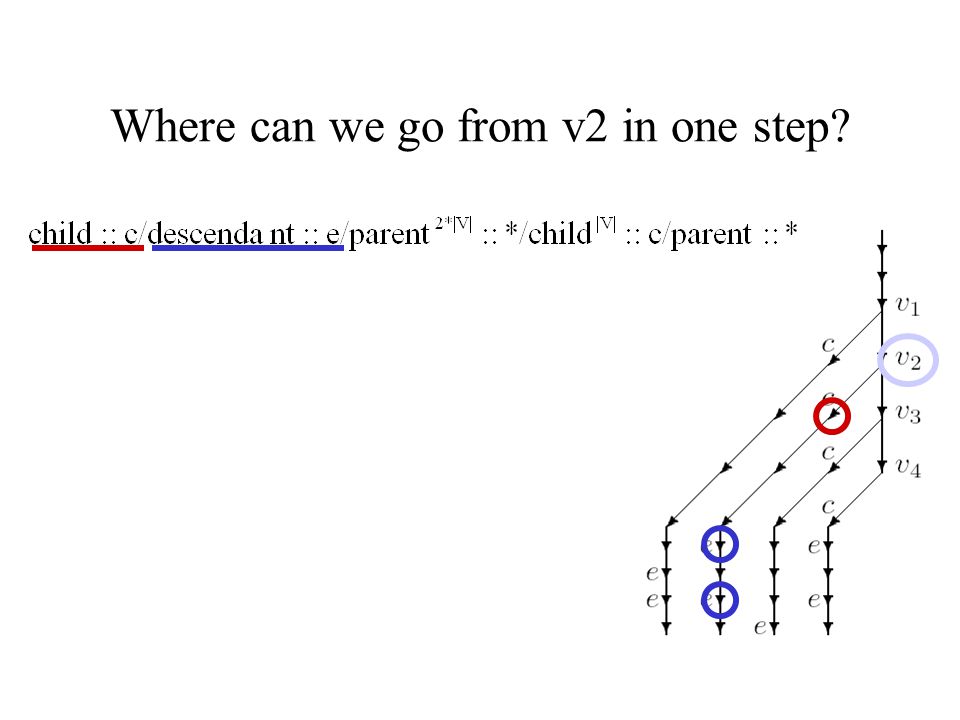
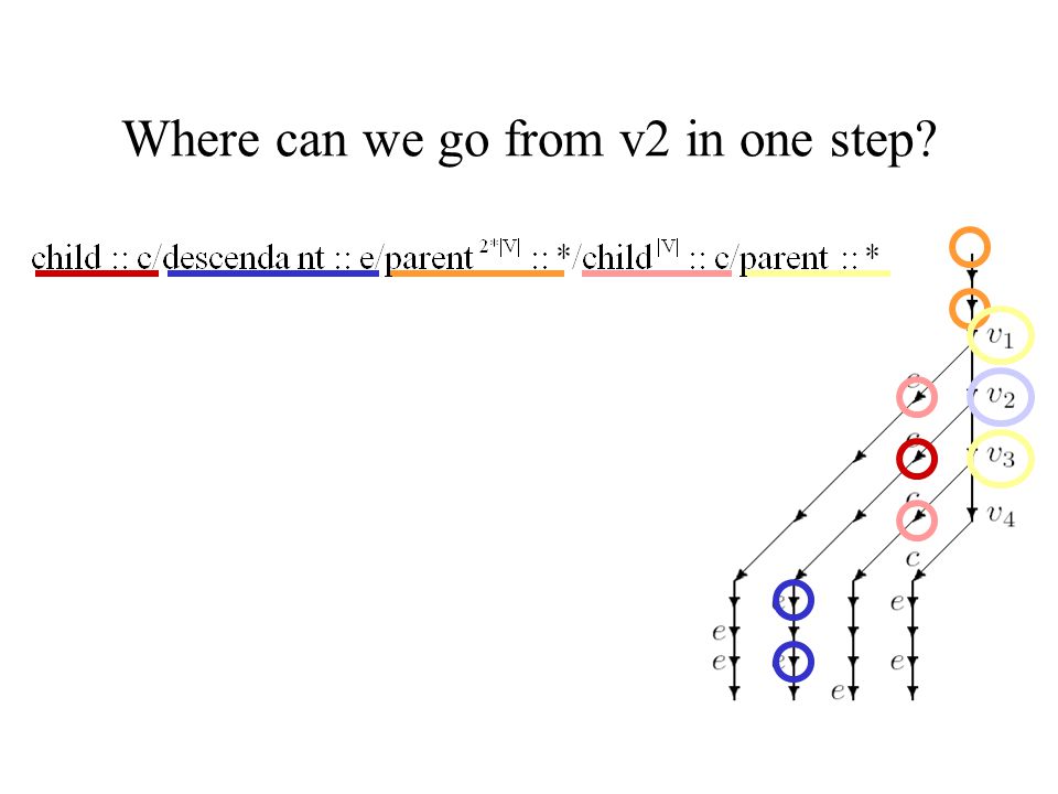
11. PF – Path Query Fragment PF = Core XPath without conditions. E.g. //a/b//c/parent::d//f/g/ancestor::a/* Theorem: PF is NL-complete w.r.t. combined complexity (and L- reductions). Membership: paths easy to guess and check in NL. NL-Hardness by reduction from Graph Reachability …

13. Where can we go from v2 in one step?

19. Reachable from v2 in one step: v1, v3!

20. PF is NL-hard. Reachability in precisely m steps: Add loop at each node to graph => reachability in at most m steps. Set m = |E|.

21. Further fragments with low parallel complexity Combined complexity of Core Xpath is in L if: 1.Only one-step axes are used (child, parent; self). 2.Only transitive downward axes are used (descendant, descendant-or-self, …).

22. Increasing the Size of the LOGCFL Fragment “positive Wadler fragment” [Wadler, 2000]: just like positive Core XPath, but with position arithmetics in conditions. –child::a[position()+1 = last()] … get the second-last child labeled “a”. –No iteration of predicates: child::a[…][…]. Theorem (combined complexity): the positive WF is –LOGCFL-complete; –with iterated predicates (already when iterated at most twice), it is P-complete.

23. Increasing the Size of the LOGCFL Fragment pXPath: “positive”/parallel XPath. 1.No negation 2.No iterated predicates […][…] 3.Depth of nesting of arithmetic operations inside a predicate is bounded by some constant. 4.Forbidden built-in functions: count, sum, string, local-name, name, namespace-uri, string-length, normalize-space. 5.Forbidden: relational operations on booleans. Theorem. pXPath is LOGCFL-complete (combined complexity). Maximal parallelizable fragment of Xpath, unless P = NC. –Adding any of the features (1) – (5) leads to P-hardness.

24. Combined Complexity of XPath

25. Data and Query Complexity Theorem. PF is L-complete under NC1-reductions (data complexity). Theorem. XPath w/o multiplication, concatenation is in L w.r.t. query complexity. Surprisingly, data complexity and query complexity are low; combined complexity is higher! L L-complete (NC1-red.) XPath PF Data complexity

26. Processing Xpath on Streams using Finite Automata

27. FSA on Streams Translate Xpath path query into FSA, process stream of (e.g.) SAX events. –Very good scalability, low memory consumption (stack needed) Selective dissemination of information (SDI) / publish-subscribe (cf. Xfilter [Altinel and Franklin, VLDB 2000], Xtrie [Chan et al., ICDE 2002]). –Boolean queries. –Extensions to support branching tree patterns, condition predicates, backward axes, … –Goal is to evaluate multiple queries at once (10^4 – 10^6 queries.)

28. Example: $x in //a/b a b aab ab b $x NFADFA (0)

29. Example: //a/b a b aab ab b $x NFADFA (0) (01)

30. Example: //a/b a b aab ab b $x NFADFA (0) (01)

31. Example: //a/b a b aab ab b $x NFADFA (0) (01) (02) $x

32. Example: //a/b a b aab ab b $x NFADFA (0) (01) $x

33. Example: //a/b a b aab ab b $x NFADFA (0) (01) $x

34. Example: //a/b a b aab ab b $x NFADFA (0) (01) $x (01)

35. Example: //a/b a b aab ab b $x NFADFA (0) (01) $x

36. Example: //a/b a b aab ab b $x NFADFA (0) (01) $x (02) $x

37. Example: //a/b a b aab ab b $x NFADFA (0) (01) $x (02) $x (01)

38. Example: //a/b a b aab ab b $x NFADFA (0) (01) $x (02) $x (01) (02) $x

39. Example: //a/b a b aab ab b $x NFADFA (0) (01) $x (02) $x (01) $x

40. Example: //a/b a b aab ab b $x NFADFA (0) (01) $x (02) $x

41. Example: //a/b a b aab ab b $x NFADFA (0) (01) $x

42. Example: //a/b a b aab ab b $x NFADFA (0) $x

43. Size of DFAs //a/*/*/b

44. Size of DFAs Exponential in the size of Xpath statement, but –Only exponential in number of occurrences of “*”. –In case of automaton for multiple queries, exponential in number of occurrences of “//”. Lazy evaluation of DFA –Computation of states and transitions only on demand. –Saves much time and space in practice: documents usually from quite restrictive language. [Green, Miklau, Onizuka, Suciu, ICDT 2003]

45. Extensions Branching tree patterns. Condition predicates. Backward axes Boolean queries (“Can tree pattern be embedded into XML document?”) –Rather than node-selecting queries.

46. Highly Expressive Queries and Automata

47. Motivation Scalability in databases = (all three points at the same time) –Strictly linear time. –Little main memory required (DB in secondary storage). –Little jumping around in the data, sequential scans of disk preferred (streaming). Paged sequential reading much faster than random access. Node-selecting queries on unranked trees (XML) –Higher expressiveness than what is possible with single pass. Folklore: unary MSO queries can be evaluated in two passes through the tree.

48. The Arb Query Processor Evaluates node-selecting queries –In two sequential scans of the data. –Memory requirements: O(depth(tree)), otherwise independent of size of DB. –Highly parallelizable. –Tree Automata-based. –High expressiveness: unary Monadic Second Order Logic (MSO). –Succinct representation of automata. [Frick, Grohe, K., LICS 2003; K., VLDB 2003]

49. Selecting Tree Automata (STAs) STA: Nondeterministic bottom-up tree automata with a set of selecting states. Select a node if it is assigned a selecting state in all (or one) accepting runs: or Expressive power: unary MSO queries on trees. [Neven’s thesis]; [Frick, Grohe & K., LICS 2003]

50. Two-Phase Query Evaluation From STA 1.Deterministic bottom-up tree automaton –compute reachable states. 2.Deterministic top-down tree automaton (with selection) Eliminate state-to-node assignments that do not lead to accepting run. Select nodes of query result. [Frick, Grohe & K., LICS 2003]

51. Representation on Disk

52. a b ba a ccc b bb ba a

53. a b ba a ccc b bb ba a FirstChildNextSibling

54. Representation on Disk 1 23 45691112 78 1013 14 a b ba a ccc b bb ba a FirstChildNextSibling

55. Representation on Disk 1 23 45691112 78 1013 14 1 2 3 4 5 6 7 8 9 10 11 12 13 14 10011101 00011101 00 abaabcbabccabbLabel: Children? a b ba a ccc b bb ba a FirstChildNextSibling

56. Running Automata by Sequential Disk Scans

57. Running Automata by Seq. Scans Deterministic top-down tree automaton –One sequential forward scan of the data. –Memory: Stack bounded by depth of tree. Deterministic bottom-up tree automaton –One sequential backward scan of the data. –Memory: Stack bounded by depth of tree. For unranked trees !

58. Bottom-up Traversal 1 23 45691112 78 1013 14 1 2 3 4 5 6 7 8 9 10 11 12 13 14 14 10011101 00011101 00

59. Bottom-up Traversal 1 23 45691112 78 1013 14 1 2 3 4 5 6 7 8 9 10 11 12 13 14 14 10011101 00011101 00

60. Bottom-up Traversal 1 23 45691112 78 1013 14 1 2 3 4 5 6 7 8 9 10 11 12 13 14 14 10011101 00011101 00 13

61. Bottom-up Traversal 1 23 45691112 78 1013 14 1 2 3 4 5 6 7 8 9 10 11 12 13 14 14 13 10011101 00011101 00

62. Bottom-up Traversal 1 23 45691112 78 1013 14 1 2 3 4 5 6 7 8 9 10 11 12 13 14 14 13 10011101 00011101 00

63. Bottom-up Traversal 1 23 45691112 78 1013 14 1 2 3 4 5 6 7 8 9 10 11 12 13 14 14 10011101 00011101 00 12

64. Bottom-up Traversal 1 23 45691112 78 1013 14 1 2 3 4 5 6 7 8 9 10 11 12 13 14 14 12 10011101 00011101 00

65. Bottom-up Traversal 1 23 45691112 78 1013 14 1 2 3 4 5 6 7 8 9 10 11 12 13 14 14 10011101 00011101 00 11

66. Bottom-up Traversal 1 23 45691112 78 1013 14 1 2 3 4 5 6 7 8 9 10 11 12 13 14 14 10011101 00011101 00 10

67. Bottom-up Traversal 1 23 45691112 78 1013 14 1 2 3 4 5 6 7 8 9 10 11 12 13 14 14 10011101 00011101 00 9

68. Bottom-up Traversal 1 23 45691112 78 1013 14 1 2 3 4 5 6 7 8 9 10 11 12 13 14 14 10011101 00011101 00 9

69. Bottom-up Traversal 1 23 45691112 78 1013 14 1 2 3 4 5 6 7 8 9 10 11 12 13 14 8 10011101 00011101 00

70. Bottom-up Traversal 1 23 45691112 78 1013 14 1 2 3 4 5 6 7 8 9 10 11 12 13 14 7 10011101 00011101 00

71. Bottom-up Traversal 1 23 45691112 78 1013 14 1 2 3 4 5 6 7 8 9 10 11 12 13 14 7 10011101 00011101 00 6

72. Bottom-up Traversal 1 23 45691112 78 1013 14 1 2 3 4 5 6 7 8 9 10 11 12 13 14 7 10011101 00011101 00 5

73. Bottom-up Traversal 1 23 45691112 78 1013 14 1 2 3 4 5 6 7 8 9 10 11 12 13 14 7 10011101 00011101 00 4

74. Bottom-up Traversal 1 23 45691112 78 1013 14 1 2 3 4 5 6 7 8 9 10 11 12 13 14 3 10011101 00011101 00

75. Bottom-up Traversal 1 23 45691112 78 1013 14 1 2 3 4 5 6 7 8 9 10 11 12 13 14 2 10011101 00011101 00

76. Bottom-up Traversal 1 23 45691112 78 1013 14 1 2 3 4 5 6 7 8 9 10 11 12 13 14 1 10011101 00011101 00

77. Monadic Datalog and TMNF Monadic datalog: datalog, all “intensional predicates” are unary. Over unranked, ordered, finite trees: –Unary: Root, hasFirstChild, hasNextSibling, Label_a, and their complements. –Binary: FirstChild, NextSibling Example: D0(x) :- Root(x). D1(x) :- D0(x0), First-Child(x0, x). D0(x) :- D1(x0), First-Child(x0, x). D0(x) :- D0(x0), Next-Sibling(x0, x). D1(x) :- D1(x0), Next-Sibling(x0, x). TMNF (“tree-marking normal form”) - restricted syntax: –P(x) :- P1(x), P2(x). P(x) :- P0(x0), R(x0, x). P(x) :- P0(x0), R(x, x0). D0: nodes at even depth in tree. D1: nodes at odd depth in tree.

78. Known Facts about Monadic Datalog [Gottlob & K., PODS 2002]: M.dl.o.t. can be evaluated in time O(|Program| * |Data|). M.dl.o.t. captures the unary MSO queries over trees. [Gottlob & K., LICS 2002], [Frick, Grohe, K. LICS 2003]: Linear-time reduction to TMNF. Linear-time reduction also from Core Xpath to TMNF (negation!) [Grohe and Schweikardt, CSL 2003]: But: M.dl. much less succinct than MSO, monadic fixpoint logic. –However, no problems observed in practice yet.

79. TMNF Example P1(x) :- Root(x). P2(y) :- P1(x), FirstChild(x,y). P3(y) :- P2(x), FirstChild(x,y). P4(y) :- P3(x), FirstChild(y, x). P5(y) :- P4(x), FirstChild(y, x). {P1} {}

80. TMNF Example P1(x) :- Root(x). P2(y) :- P1(x), FirstChild(x,y). P3(y) :- P2(x), FirstChild(x,y). P4(y) :- P3(x), FirstChild(y, x). P5(y) :- P4(x), FirstChild(y, x). {P1} {P2} {}

81. TMNF Example P1(x) :- Root(x). P2(y) :- P1(x), FirstChild(x,y). P3(y) :- P2(x), FirstChild(x,y). P4(y) :- P3(x), FirstChild(y, x). P5(y) :- P4(x), FirstChild(y, x). {P1} {P2} {P3}

82. TMNF Example P1(x) :- Root(x). P2(y) :- P1(x), FirstChild(x,y). P3(y) :- P2(x), FirstChild(x,y). P4(y) :- P3(x), FirstChild(y, x). P5(y) :- P4(x), FirstChild(y, x). {P1} {P2,P4} {P3}

83. TMNF Example P1(x) :- Root(x). P2(y) :- P1(x), FirstChild(x,y). P3(y) :- P2(x), FirstChild(x,y). P4(y) :- P3(x), FirstChild(y, x). P5(y) :- P4(x), FirstChild(y, x). {P1,P5} {P2,P4} {P3}

84. Implementation Bottom-up phase has to deal with nondeterminism – very large sets of states possible. Compact representation of state sets using residual logic programs. Compilation of TMNF program P into –Deterministic bottom-up automaton Sets of reachable states of STA become states of. Each such state is represented as a residual logic program. –Deterministic top-down automaton. Both evaluated lazily: Transitions computed on demand and stored.

85. Propositional “Local” Program P1(x) :- Root(x). P2(y) :- P1(x), FirstChild(x,y). P3(y) :- P2(x), FirstChild(x,y). P4(y) :- P3(x), FirstChild(y, x). P5(y) :- P4(x), FirstChild(y, x). P1 :- Root. P2[1] :- P1. P3[1] :- P2. P4 :- P3[1]. P5 :- P4[1]. “Local” [1][2]

86. Bottom-up Run P1 :- Root. P2[1] :- P1. P3[1] :- P2. P4 :- P3[1]. P5 :- P4[1]. A

87. Bottom-up Run P1 :- Root. P2[1] :- P1. P3[1] :- P2. P4 :- P3[1]. P5 :- P4[1]. A {}

88. Bottom-up Run {} P1 :- Root. P2[1] :- P1. P3[1] :- P2. P4 :- P3[1]. P5 :- P4[1]. A

89. Bottom-up Run {} {P4 :- P2} P1 :- Root. P2[1] :- P1. P3[1] :- P2. P4 :- P3[1]. P5 :- P4[1]. A Represents 2^3 * (2^2 - 1) = 24 reachable states

90. Bottom-up Run {} P1 :- Root. P2[1] :- P1. P3[1] :- P2. P4 :- P3[1]. P5 :- P4[1]. {P4 :- P2} A + {Root; P4[1] :- P2[1]}

91. Bottom-up Run {} P1 :- Root. P2[1] :- P1. P3[1] :- P2. P4 :- P3[1]. P5 :- P4[1]. {P4 :- P2} A + {Root; P4[1] :- P2[1]} {P1; P2[1]; P4[1]; P5}

92. Top-down Run {} P1 :- Root. P2[1] :- P1. P3[1] :- P2. P4 :- P3[1]. P5 :- P4[1]. {P4 :- P2} A {P1; P2[1]; P4[1]; P5}

93. Top-down Run {} P1 :- Root. P2[1] :- P1. P3[1] :- P2. P4 :- P3[1]. P5 :- P4[1]. {P4 :- P2} A {P1; P2[1]; P4[1]; P5} + {P2; P4}

94. Top-down Run {} P1 :- Root. P2[1] :- P1. P3[1] :- P2. P4 :- P3[1]. P5 :- P4[1]. {P2; P3[1]; P4} A {P1; P2[1]; P4[1]; P5} + {P2; P4}

95. Top-down Run {} P1 :- Root. P2[1] :- P1. P3[1] :- P2. P4 :- P3[1]. P5 :- P4[1]. A {P1; P2[1]; P4[1]; P5} + {P3} {P2; P3[1]; P4}

96. Top-down Run {P3} P1 :- Root. P2[1] :- P1. P3[1] :- P2. P4 :- P3[1]. P5 :- P4[1]. A {P1; P2[1]; P4[1]; P5} + {P3} {P2; P3[1]; P4}

97. Encode string as almost complete binary “infix” tree. Represent backward step between leaves as caterpillar (tree- walking) expression. Express regular expression over strings as monadic datalog program over infix tree. Example: Parallel Regular Expression Matching e x a m p l e

98. Some further interesting work Structural Joins, Twig Joins –[Al-Khalifa et al., ICDE 2002; Bruno, Koudas, and Srivastava, SIGMOD 2002; …] –Exploit tree structure to compute matches of tree pattern in time O(|input| + |output|). Index Structures for Path Expressions –[Kemper and Moerkotte, 1992; Milo and Suciu, ICDT 1999] –Bisimulation; data guides, 1-indexes, t-indexes, … Optimization of XPath –Containment and Minimization [Miklau and Suciu, PODS 2002, Neven and Schwentick, ICDT 2003; Wood, WebDB 2001, ICDT 2003; Deutsch and Tannen, KRDB 2001] –Satisfiability [Hidders, DBPL 2003] –Axiom sytems for query rewriting [Benedikt, Fan and Kuper, ICDT 2003] Closure Properties for Xpath Fragments –[Benedikt, Fan and Kuper, ICDT 2003]

99. END