1. CLIC CDR Schedules & Value Estimates Philippe Lebrun on behalf of the CLIC Cost & Schedule WG LCWS 12 University of Texas at Arlington, USA 22 – 26 October 2012

2. Contents Scope of the CLIC CDR study Construction & operation schedules Value estimate methodology Uncertainty & risk Escalation & exchange rate fluctuations CDR value estimates Potential for cost reduction

3. Contents

4. Scope of the CLIC CDR study CDR Volume 1 The basic parameters for the CLIC CDR study are optimized for a collision energy of 3 TeV and a peak luminosity of 2 E34 cm -2 s -1 The study includes a first stage at 500 GeV, for which a single drive-beam production complex is sufficient to power both main linacs The bunch charge must be almost doubled to preserve luminosity at 500 GeV. This results in –Main linac accelerating structures with larger iris and lower gradient (80 MV/m) –Longer main linacs (2 x 5 sectors) –Increased RF power in the drive-beam and main-beam production complexes The schedule aims at reaching the 3 TeV stage as early as permitted by civil construction and machine installation constraints: operation at 500 GeV only occurs in the shade of the 3 TeV construction schedule Supply of series components matches the dates of availability for installation of the 3 TeV stage, thus demanding high production rates and corresponding fixed costs Industrial contracts for production of series components are established from the onset for the 3 TeV quantities, to benefit from extended learning curves and lower average unit costs

5. CLIC layout at 3 TeV

6. CLIC layout at 500 GeV

7. Scope of the CLIC CDR study Changes in CDR Volume 3 [1/3] Introduction of an intermediate energy stage –Physics case may require collision energy at or above 1 TeV –Introduction of intermediate energy stage is the optimum approach for covering the full range of collision energy with sufficient luminosity –The stepwise increase in cost/complexity resulting from the second drive- beam complex leads to choose this intermediate stage at around 1.5 TeV

8. Value estimate vs energy Scope of the CDR study Value E cm 3 TeV ultimate 500 GeV as phase 1 of ultimate 3 TeV (one DB complex) 500 GeV optimized (under study) 1.5 TeV as phase 2 (one DB complex) Cost of 2 nd DB complex

9. Scope of the CLIC CDR study Changes in CDR Volume 3 [2/3] Inclusion of operation schedule driven by physics requirements and expected machine performance –Integrated luminosity goals of 500 fb -1 at 500 GeV, 1.5 ab -1 at ~1.5 TeV, and 2 ab -1 at 3 TeV –Operational efficiency (collider & detectors) taken at 0.5 for 200 days/year, with ramp-up in the first years of each stage –As a consequence, the complete program develops over >20 years, well beyond the horizon of any industrial contract –The supply of series components must now only match the dates of availability for installation of each stage, leading to production rates ~3 times lower (and thus lower fixed costs) –The industrial production contracts of series components only concern quantities corresponding to each stage, leading to shorter learning curves and thus higher average unit costs

10. Operation for physics Integrated luminosity targets –500 fb -1 at 500 GeV –1.5 ab -1 at 1.4/1.5 TeV –2 ab -1 at 3 TeV Luminosity ramp-up –Four years in first stage –Two years in subsequent stages

11. Production of accelerating structures G. Riddone

13. Scope of the CLIC CDR study Changes in CDR Volume 3 [3/3] Two alternative staging scenarios –Each with three stages: 500 GeV, ~1.5 TeV and 3 TeV –Scenario A: « optimized for luminosity in the first stage » –Scenario B: « optimized for lower entry cost » –First and last stages of scenario A are identical to CDR Volume 1 –Reuse of 80 MV/m structures in scenario A limits the energy of the second stage to 1.4 TeV –Scenario B has nominal bunch charge at all stages, resulting in Use of final (100 MV/m) gradient structures already at 500 GeV Shorter main linacs (2 x 4 sectors) Lower installed RF power in the main-beam and drive-beam production complexes

14. Parameters for Scenario A « optimized for luminosity at 500 GeV »

15. Parameters for Scenario B « lower entry cost »

16. Upgrade paths for both Scenarios Scenario A Scenario B

17. CLIC footprints near CERN

18. Contents

19. Operation for physics Integrated luminosity targets for physics –500 fb -1 at 500 GeV –1.5 ab -1 at 1.4/1.5 TeV –2 ab -1 at 3 TeV

20. Progress rate assumptions Civil engineering –site installation: 15 weeks –shaft excavation and concrete: 180 m deep: 30 weeks 150 m deep: 26 weeks 100 m deep: 15 weeks –service caverns: 35 weeks –excavation by tunnel-boring machine (TBM): 150 m/week Installation of general services –Survey & floor markings: 9 weeks/km/front –electrical general services: 8 weeks/km/front –cooling pipes & ventilation ducts: 8 weeks/km/front –AC and DC cabling: 8 weeks/km/front Installation of main linacs –Transport of two-beam modules: 500/month –Interconnection of two-beam modules: 300 to 400/month

21. Main linac construction schedule – Scenario A K. Foraz Years K. Foraz

22. Main linac construction schedule – Scenario B K. Foraz Years K. Foraz

23. Interaction region schedule M. Gastal

24. Overall construction schedule - Scenario A K. Foraz Years

25. Overall construction schedule - Scenario B K. Foraz Years

26. Contents

27. Value, explicit labor & cost CLIC will be a global project –with contributions in different forms (in-cash, in-kind, in personnel) –from different regions of the world –using different accounting systems « Value & explicit labor » methodology –independent of any particular accounting system –compatible with this diversity –adopted by ITER, ILC RDR Value –lowest reasonable estimate of the price of goods and services procured from industry on the world market in adequate quality and quantity –expressed in CHF of December 2010 Explicit labor –personnel provided by central laboratory and collaborating institutes –expressed in person.years

28. Value estimates are given in December 2010 CHF 1 EUR = 1.28 CHF 1 USD = 0.96 CHF 1 JPY = 0.0116 CHF Euro to Swiss franc US dollar to Swiss franc

29. Scope of the value estimate Included –« Project construction » costs, i.e. from project approval to commissioning with beam –DB injector complex, MB injector complex, main linacs, infrastructure for experiments, beam disposal –Specific tooling dedicated for production of components –Reception tests and pre-conditioning of components –Commissioning of technical systems (w/o beam) –« Explicit labor » including dedicated services e.g. project office, monitoring & oversight of collaborations: counted separately Excluded –R&D, prototyping & pre-industrialization –Land acquisition & underground rights-of-way –Detectors –Computing –General laboratory infrastructure e.g. library, fire brigade, hostel, cafeteria –General laboratory services, e.g. administration, human resource management, purchasing, finance, communication & outreach –Commissioning with beam, operation, decommissioning –Spares (charged to operations budget) –Taxes & custom duties

30. Value estimate follows PBS/WBS Level 2 PBS/WBSDomain coordinatorsLevel 1 PBS/WBS

31. PBS/WBS levels Architecture –Level 1: Domain Main beam production –Level 2: Subdomain Injectors –Level 3: Component Pre-injector linac for e- Multiplicities of components included –Level 4: Technical systemRF system List standardized –Level 5: SubcomponentKlystron Depending upon type of domain and estimation method, elementary value estimates entered at level of component, technical system or subcomponent

32. Value estimate methods Analytical –Based on project/work breakdown structure –Define production techniques –Estimate fixed costs –Establish unit costs & quantities (including production yield and rejection/reprocessing rates) –In case of large series, introduce learning curve (see later) Scaling –Establish scaling estimator(s) and scaling law(s), including conditions & range of application Empirical « First-principles » based –Define reference project(s) and fit data In most cases, hybrid between these methods

33. CLIC Study Costing Tool CLIC Study Costing Tool developed & maintained by CERN GS-AIS Operational, on-line from C&S WG web page (access protected) Includes features for currency conversion, price escalation and uncertainty Production of cross-tab reports exportable to EXCEL Full traceability of input data

34. CLIC two-beam modules Complexity, number, integration G. Riddone CLIC at 500 GeV (4’232 modules) 26’920 Accelerating Structures 13’460 PETS ~ 70’000 RF components CLIC at 1.5 TeV (10’730 modules) 71’380 Accelerating Structures 35’690 PETS ~ 200’000 RF components

35. Learning curves: from airplanes to accelerator components T.P. Wright, Factors affecting the cost of airplanes, Journ. Aero. Sci. (1936) Unit cost c(n) of nth unit produced c(n) = c(1) n log 2 a with a = « learning percentage », i.e. remaining cost fraction when production is doubled Cumulative cost of first nth units C(n) = c(1) n 1+log 2 a / (1+log 2 a) with C(n)/n = average unit cost of first nth units produced n = number per production line ≠ total number in project  verified on LHC main magnets up to series of  400 units/manufacturer

36. Learning coefficients P. Fessia

37. Ph. Lebrun – EURONu Workshop Effect of learning coefficient on average unit cost up to rank N

38. Saturation of learning process has little impact on total cost

39. Contents

40. Ph. Lebrun - 100426 Cost variance factors and how to handle them Technical design –Evolution of system configuration –Maturity of component design –Technology breakthroughs –Variation of applicable regulations Industrial execution –Qualification & experience of vendors –State of completion of R&D, of industrialization –Series production, automation & learning curve –Rejection rate of production process Structure of market –Mono/oligopoly –Mono/oligopsone (one-off supply) Commercial strategy of vendor –Market penetration –Competing productions Inflation and escalation –Raw materials –Industrial prices International procurement –Exchange rates –Taxes, custom duties Engineering judgement of responsible Tracked and compensated Decreasing control of project responsible Outside project control Procurement Contract adjudication Technical definition Reflected in scatter of offers received from vendors (LHC experience)

41. Ph. Lebrun - 100426 Observed tender prices for LHC accelerator components Adjusted to mean (1.46) and total number (218) of sample

42. Lowest-bidder from n valid offers Analytical solution –Consider two valid offers X1, X2 following same exponential distribution with P(Xi<x) = F(x) = 1 – exp[-a(x-b)] ⇒ m = b + 1/a and  = 1/a –Price paid (lowest valid offer) is Y = min(X1, X2): what is the probability distribution of Y? –Estimate P(Y<x) = P(X1<x or X2<x) = G(x) –Combined probability theorem P(X1<x or X2<x) = P(X1<x) + P(X2<x) – P(X1<x and X2<x) –If X1 and X2 uncorrelated, P(X1<x and X2<x) = P(X1<x) * P(X2<x) –Hence, P(X1<x or X2<x) = P(X1<x) + P(X2<x) – P(X1<x) * P(X2<x) and thus G(x) = 2 F(x) – F(x) 2 = 1 – exp[-2a(x-b)] ⇒ Y follows exponential distribution with m = b + 1/2a and  = 1/2a –By recurrence, if n uncorrelated valid offers X1, X2,…Xn are received, the price paid Y = min (X1, X2,…Xn) will follow an exponential distribution with m = b + 1/na and  = 1/na Monte Carlo simulation –Produce 400 random drawings of sets of n values of X distributed according to F(x) –For each set, take Y = min(X1, X2,..Xn) and estimate mean and std dev of 400 realizations of Y –Monte Carlo simulation in accordance with analytical solution

43. Sampling from LHC tender price distribution to estimate lowest-bidder price vs number of offers

44. Method for CLIC value risk assessment 1. For each value element k Separate value risk factors in three classes, assumed independent –Technical design maturity & evolution of configuration Represented by relative standard deviation  technical (k) Rank in three levels yielding different values of  technical (k) –Known technology  0.1 –Extrapolation from known technology0.2 –Requires R&D0.3 –Price uncertainty in industrial procurement Represented by relative standard deviation  purchase (k) Assume lowest-bidder purchasing rule Estimate n number of valid offers to be received Apply  purchase (k) = 0.5/n –Economical & financial context Risk outside project value assessment Deterministic, compensated a posteriori by adequate indexation Estimate risk on value c(k) of element k –  c technical (k) =  technical (k) x c (k) –  c purchase (k) =  purchase (k) x c (k) –  c total (k) is the r.m.s. sum of  c technical (k) and  c purchase (k)

45. Method for CLIC value risk assessment 2. For total project Value estimate of project C =  c(k) Uncertainties  C technical =   c technical (k)  C purchase =   c purchase (k)  C total =   c total (k) Estimate uncertainty band on project value estimate [C -  C technical ; C +  C total ]

46. Contents

47. Exchange rates and cost escalation Exchange rate fluctuations should ideally reflect evolution of purchasing power of currencies, but –Economic parities offset by financial effects –Variety of escalation indices in each currency Choose « reference currency » (CHF) and apply relevant escalation indices in reference country (Office Fédéral de la Statistique, Bern) Currency A Time 1 Currency B Time 1 Exchange rate 1 Currency A Time 2 Currency B Time 2 Exchange rate 2 Escalation Index a Escalation Index b ?

48. Why not use PPPs for comparing contract prices for global accelerator construction PPPs are used to compare prices for the same goods/services in different countries constituting separate markets They are therefore not good comparative indicators of the value, i.e. the lowest reasonable estimate of the price of goods and services procured from industry on the world market Example 1: commodities –World prices of commodities (e.g. oil or… niobium) are usually quoted in single currency, often USD  relevant is the exchange rate to the USD Example 2: specific supplies such as accelerator components –Consider a producer from a low-income region: on this market, the equilibrium price for a given good/service will be lower than that in a high-income country, the ratio of these equilibrium prices is – by definition – the PPP for this good/service –When this producer enters the world market, e.g. to answer an invitation to tender from the Linear Collider Project, he will be tempted to maximize his profit by raising his price up to just below the world market equilibrium price, well above the equilibrium price in the low-income region which constitutes his usual market: the value of the supply will then be very different from the price in local currency converted by the PPP

49. Eurostat-OECD recommendations on the use of PPPs

50. Method for indexation of CLIC value estimate Economical & financial effects are compensated a posteriori –Choice of CHF as reference currency –Applications of compound indices in CHF from Office Fédéral de la Statistique (CH) Arts et métiers – Industrie for technical components Construction for civil engineering This compensation is –assumed to be granted by the funding agencies on a yearly basis on the yet unspent part of the budget –therefore outside the value risk of the project

51. Swiss vs CERN indices

52. Contents

53. Review of CLIC CDR value estimates The study of the CLIC CDR value estimates developed over 2009-2011 Scope, methodology and results were presented to an international review panel in February 2012 The comments and recommendations of the review panel were taken into consideration to modify the February 2012 value estimates and produce the revised numbers presented hereafter, in particular by –inclusion of staging scenario B –basing unit costs on results of industrial studies, whenever possible –limiting learning curve horizon to 500 GeV quantities –estimating separately and rms summing uncertainties pertaining to technical and procurement risks, deemed statistically independent

54. Value estimate CLIC 500 GeV A [CHF Dec 2010]

55. Value estimate CLIC 500 GeV B [CHF Dec 2010]

56. Value by PBS/WBS domain 8.3 +1.9 -1.4 BCHF 7.4 +1.7 -1.3 BCHF

58. A first look at personnel resources Personnel [FTE.years] –Defined as « Explicit Labor » in ILC RDR –Staff+Fellows+Associates in home laboratory & collaborating institutions –Categories: « Scientific » & « Technical » –Industrial labor charged to Material Value estimate Analytical estimate –Provide technical system responsibles with WP description, project schedule and boundary conditions, and collect estimates from them –Not applied here Global scaling from previous projects –Ratio of FTE.year to Material Value for several large accelerator projects appears slowly decreasing with increasing Material Value > few BCHF –Assume Ratio remains about constant from LHC upwards –Analyse LHC data and scale to CLIC

59. 1.9 FTE.year/MCHF

60. LHC personnel expenditure Source: periodic reports to CERN Finance Committee

61. Scaling personnel from LHC to CLIC LHC accelerator, injectors and technical areas –Included: construction, installation and pre-operation –Not included: R&D, commissioning with beam, operation –P ~ 7000 FTE.years => P/M ~ 1.9 FTE.year/MCHF 2010 –About 40% scientific, 60% technical Scaling to CLIC @ 500 GeV –Assume P/M ratio is the same as for LHC construction Scenario A15700 FTE.years Scenario B14100 FTE.years

62. Contents

63. Breakthrough vs gradual progress The case of human genome sequencing Sanger-based chemistry Capillary-based instruments Ligation chemistry Nanopore technology

64. Cost mitigation alternatives CDR cost drivers –A number of cost drivers have already been identified in the CDR phase, with cost mitigation alternatives. Some of these could already be studied and validated, and are implemented in the CDR and its value estimate. Others will be studied in the post-CDR phase –The maximum savings potential identified through this process is ~ 12% of the total value (500 GeV) Revision of basic parameters –The CLIC CDR study describes a machine optimized for the ultimate CM energy of 3 TeV, with a first stage at 500 GeV CM and a second one at 1.5 TeV CM. As a consequence, a number of technical choices for the lower energy stages are dictated by the optimization at ultimate energy, thus strongly impacting the cost of the lower energy stages. –Revising the CM energy chosen for CLIC technical optimization, while preserving the potential to reach ultimate energy, is expected to provide the main lever for cost reduction. This process has started

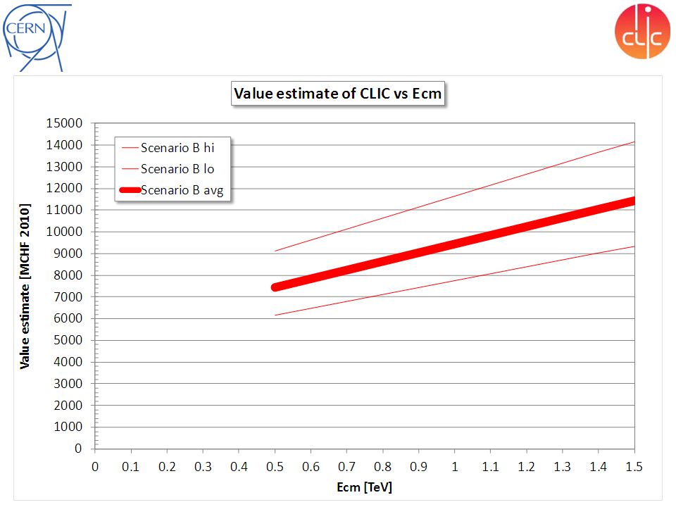
65. Conclusions Value estimates for first stage at 500 GeV CM (alternative scenarios A and B) of CLIC with ultimate 3 TeV CM –Based on PBS/WBS –Established by scientists & engineers having technical responsibility of PBS/WBS domains/subdomains, from unit data produced by technology groups –Reviewed by international panel of experts in February 2012 –Uncertainty stemming from technical and commercial unknowns estimated according to normalized procedure to [-17 %; +23 %] Variation with CM energy –Indicates large zero offset for MB and DB production complexes –Scaled value for CLIC at 1.5 TeV CM gives access to incremental cost above 500 GeV of ~4 MCHF/GeV CM Personnel (« explicit labor ») estimated globally by scaling wrt LHC –First approach to be refined by analytical estimate Cost drivers and potential for cost reduction identified – Incremental cost mitigation actions identified on components/systems, totalling at maximum ~ 12% – Major effect expected from re-optimization of basic parameters for E CM << 3 TeV