1. Here we add more independent variables to the regression.
Multiple Regression
Here we add more independent variables to the regression.

2. Let’s begin with an example of simple linear regression
Let’s begin with an example of simple linear regression. A trucking company is interested in understanding what is going on with the time the drivers are on the road. Travel time is the dependent variable. It seems that travel time would be influenced by miles traveled, the independent variable.
I have the simple regression results from such a study on the next slide.

3. Note the estimated equation is
y (time) = x(miles).
The p-value on the slope coefficient (miles line) is and since it is less than .05 we reject the null of a zero slope and conclude there is a relationship between miles driven and travel time.
R square = .66 and thus 66% of the variation in y is explained by x.
Miles time (hours)

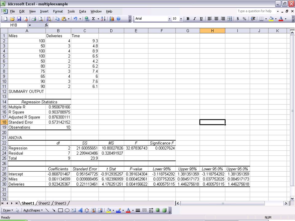
4. So, we had a significant relationship between x and y and the r-square was This r square is not bad, but the company may think that with only 66% of the variation in travel time explained by miles driven, maybe other variables will explain the variability as well. Another variable that could explain the travel time is the number of deliveries that are made. (I think in the example that travel time really means how long did it take to make the days deliveries.)
In a multiple regression we can add another variable to the initial x variable we had included.
In Excel you just include in the definition of x two (or more columns) variables Note you may want to have the y variable in the last column of the right or the first column on the left because the x’s need to be included together in contiguous columns. I have a multiple regression output on the next slide.

6. Math form The multiple regression form of the model is:
y = B0 + B1 x1 + B2x2 + … + e,
where
B0 is the y intercept of the line, Bi is the slope of the line in terms of xi, and e is an error term that captures all those influences on y not picked up by the x’s. The error term reflects the fact that all the points are not directly on the line.
So, we think there is a regression line out there that expresses the relationship between x’s and y. We have to go find it. In fact we take a sample and get an estimate of the regression line.

7. When we have a sample of data from a population we will say in general the regression line is estimated to be ^
y = b0 + b1 x1 + b2x2 + …, where the ‘hat’ refers to the estimated value of y.
Once we have this estimated line we are right back to algebra. y hat values are exactly on the line.
Now, for an each value of x we have data values, called y’s, and we have the one value of the line, called y hat.
This part of multiple regression is very similar to simple regression. But our interpretation will change a little.

8. From the multiple regression output we see the coefficients section means the estimated regression line is estimated to be
y hat = x x2.
From the simple regression we had
y hat = x1. You will note the variable x1 does not have the same value in each case.
In the simple regression case the is the increase in y for each unit increase in x1, but we could not control all the other factors at work in influencing y. In the multiple case the is the increase in y when x1 increases by 1, but we have controlled for the influence that x2 has on y by including x2 in the equation.

9. Multiple Regression Interpretation

10. Correlation, Causation
Think about a light switch and the light that is on the electrical circuit. If you and I collect data about someone flipping the switch and the lights going on and off we would be able to say that there is correlation from a statistical point of view. In fact, you and I know we can say something even stronger. We can say in this case there is causation.
In the world of business (and other areas) we want to find relationships between variables. We would hope to find correlation and if we have a compelling theory maybe we could say we have causation.

11. Example
Say we are interested in crop yield on a farm. What variables are correlated with crop yield? You and I know the amount of water has been shown to have an impact on yield, as has fertilizer and soil type, among other things. In a multiple regression setting, if
y = yield,
x1 = water amount, and x2 = amount of fertilizer, the a multiple regression would be of the form
y = Bo +B1x1 + B2x2 + e and our estimated regression would be of the form
y hat = bo +b1x1 + b2x2.

12. F Test
In a multiple regression, a case of more than one x variable, we conduct a statistical test about the overall model. The basic idea is do all the x variables as a package have a relationship with the y variable? The null hypothesis is that there is no relationship and we write this in a shorthand notation as
Ho: B1 = B2 = … =0. If this null hypothesis is true the equation for the line would mean the x’s do not have an influence on y. The alternative hypothesis is that at least one of the beta’s is not zero. Rejecting the null means that the x’s as a group are related to y.
The test is performed with what is called the F test. From the sample of data we can calculate a number called the F statistic and use this value to perform the test. In our class we will have F calculated for us because it is a tedious calculation.

13. F
Under the null hypothesis the F statistic we calculate from a sample has a distribution similar to the one shown. The F test here is a one tailed test. The farther to the right the statistic we get in the sample is, the more we are inclined to reject the null because extreme values are not very likely to occur under the null hypothesis. In practice we pick a level of significance and use a critical F to define the difference between accepting the null and rejecting the null.

14. Numerator degrees of freedom = number of x’s, in general called p.
Area we make = alpha F
Critical F
To pick the critical F we have two types of degrees of freedom to worry about. We have the numerator and the denominator degrees of freedom to calculate. They are called this because the F stat is a fraction.
Numerator degrees of freedom = number of x’s, in general called p.
Denominator degrees of freedom = n – p – 1, where n is the sample size. As an example, if n = 10 and p = 2 we would say the degrees of freedom are 2 and 7 where we start with the numerator value. You would see from a book (maybe page 672 of a stats book) the critical F is 4.74 when alpha is Many times the book also has a table for alpha = .025 and .01.

16. Area we make = alpha =.05 hereF
4.74 here
In our example here the critical F is If from the sample we get an F statistic that is greater than 4.74 we would reject the null and conclude the x’s as a package have a relationship with the variable y.
On the previous slide is an example and the F stat is and so the null hypothesis would be rejected in that case.

17. Area we make = alpha =.05 hereF
4.74 here
P-value
The computer printout has a number on it that means we do not even have to look at the F table if we do not want to. But, the idea is based on the table. Here you see is in the rejection region. I have colored in the tail area for this number. Since 4.74 has a tail area = alpha = .05 here, we know the tail area for must be less than This tail area is the p-value for the test stat calculated from the sample and on the computer printout is labeled Significance F. In the example the value is

18. SOOOOOOO,
Using the F table,
Reject the null if the F stat > critical F in the table, or
If the Significance F < alpha.
If you can NOT reject the null then at this stage of the game there is no relation between the x’s and the y and our work here would be done. So from here out I assume we have rejected the null.
T tests
After the F test we would do a t test on each of the slopes similar to what we did in a simple linear regression case to make sure that each variable on its own has a relationship with y. There we reject the null of a zero slope when the p-value on the slope is less than alpha.

19. Multicollinearity
Can you say multicollinearity? Sure you can. Let’s all say it together on the count of 3. 1, 2, 3 multicollinearity! Very good class, now listen up!
Multicollinearity is an idea that volumes have been written about. We want to have a basic feel for the problem here.
You and I want x variables that help explain y. The reason is so that we can predict and explain movement in y. As an example, if we can predict and explain crop yield maybe we can make yield higher so that we can feed the world!
So, we want x’s that are correlated with y. This is a good thing. But, sometimes the x’s will be correlated with each other. This is called multicollinearity. The problem here is that sometimes we can not see the separate influence an x has on y because the other x’s have picked up the influence due to their correlation.

20. From a practical point of view multicollinearity could have the following affect on your research. You reject the null hypothesis of no relationship between all the x variables and y with the F test, but you can not reject some or all of the separate t tests for the separate slopes. Don’t freak out (yet!).
Let’s think about crop yield. Some farmers have water systems. The more it rains in a summer the less water the farmers directly apply. (Okay, maybe I am ignorant here and farmers here can use all the water they can apply – its an example.) If you included both inches of rain and water applied there is a correlation between the two. This may make it difficult to see the separate impact of either the rain or the water from the system.
If the x’s (the independent variables) have correlations more extreme than .7 or -.7 then multicollinearity could be a problem

21. r square
r square on the regression printout is a measure designed to indicate the strength of the impact of the x’s on y. The number can be between 0 and 1, with values closer to 1 meaning the stronger the relationship.
r square is actually the percentage of the variation in y that is accounted for by the x variables. This is also an important idea because although we may have a significant relationship we may not be explaining much. From the yield example the more variation we can explain then the more we can control yield and thus feed the world, perhaps. Or maybe in business setting the more variation we can explain the more profit we can make.

22. Qualitative Independent Variables
Sometimes called Dummy Variables

23. In the simple and multiple regression we have studied so far the dependent variable, y, and the independent variable(s), x(s) have been quantitative variables. But the regression can be used with other variables. We will study the case where
The dependent variable, y, is quantitative,
One (or more, in general) independent variable is quantitative, and,
One independent variable is qualitative.
Remember that a qualitative variable is of the type where different values for the variable are just categories. Some examples include gender and method of payment (cash, check, credit card).

24. An example
y = the repair time in hours. The company provides maintenance and it would like to understand why the repair time takes as long as it does. With an understanding of repair time maybe it can schedule employee hours better or improve company performance in some other way.
x1 = the number of months since the last repair service was performed. The idea is that the longer since the last repair the more that will be need to be done. The is a quantitative variable.
x2 = the type of repair service needed. In this example there are only two types of repairs – electrical and mechanical.
So, the company has clients that need repairs and the company is exploring what accounts for the time it takes to make a repair.

25. On the next slide I have a graph with two quantitative variables are on the axes. The two ovals represent the “cloud” of data points. Here the points suggest a positive relationship between months since last repair and repair time. Of course, we will have to test if this is the real case or not, but the graph suggests that is the case.
I have two ovals because it is thought that maybe each type of repair has a different impact on repair time. The different ovals represent what is happening for each type of repair and here I am suggesting that there is a difference in repair time for each level of repair type. Here we will also do a test to see if the different types of repair lead to different repair times.

26. Repair time
Months since last repair

27. The model
Here the regression model is
y = Bo +B1x1 + B2x2. When we estimate the model we use data on y and x1 and x2. Here we make the data for x2 special. We will say that x2 = 0 if the data point is for a mechanical repair and x2 = 1 if the data point is for an electrical repair.
Now, when we look at the model for the two types of repair we get the following: When x2=0
y = Bo + B1x1 + B2(0) = Bo + B1x1, and when x2 = 1,
y = Bo + B1x1 + B2(1) = Bo + B2 + B1x1. The impact of creating x2 as a 0, 1 variable is that when the value is 0 we have one line and when the value is 1 we have another line with a different intercept. The intercept is Bo with the mechanical repair and the intercept is Bo + B2 with the electrical repair.

29. Getting and interpreting the results:
The previous slide has the Excel printout for this regression model. The interpretation starts with the F test. The null is that both B1 and B2 are equal to zero. Here the F stat is with a p-value (Significance F) = Then we would reject the null with alpha as small as .001 (certainly we reject at alpha = .05) and we go with the alternative that at least one of the beta’s is not equal to zero. In other words, as a package the x’s exhibit a relationship with the y variable.
The next step is to do the t tests on each slope value B1 and B2 (even here we tend to ignore the test on Bo because we typically do not have much data with all the x’s = 0) separately. Here the p-values on both have values less than .05 so we reject the null and conclude each variable has an impact on y.

30. Repair time
Electrical y = ( ) x1
Mechanical y = x1
.9305
Months since last repair

31. On the previous slide I reproduced the graph I had before, and I added the equations for repair time under each value of x2.
When x2 = 0 we have the line for mechanical types of repair. When x2 = 1 we have the line for electrical types of repair. Ultimately the difference in the two lines here is in the intercept. But, the slope of each line is the same. This means that months since the last repair has the same impact on repair under either type of repair. Since b2 = (really since we rejected the null that B2 = 0) the electrical line has a higher intercept. We can use each equation to predict repair time given the value of months since last repair, and given the type of repair. Of course, if the type is mechanical we use the mechanical line and we use the electrical line for the electrical type.
The next thing we would do is evaluate R square. Here the value is and this indicates that just over 85% of the variation in y is explained by the x’s.

32. The qualitative variable
In our example we had a qualitative variable with two categories. Note we added 1 x variable for this 1 qualitative variable. The reason is because the 1 variable had 2 categories. Now if the 1 qualitative variable has 3 categories we would have to have 2 x variables. Say we had mechanical, electrical and industrial repair types. We would need x2 and x3 variables, in addition to repair time, x1.
With 3 categories we would have 3 lines.
When x2 = 0 and x3 = 0 the intercept would be Bo for the mechanical line.
When x2 = 1 and x3 = 0 the intercept would b Bo + B2 for the electrical line (assuming the tests had us reject the null).
When x2 = 0 and x3 = 1 the intercept would be B0 + b3 for the industrial line.

33. In general, if the 1 qualitative variable has k categories, we add k-1 x’s. When all the x’s are zero we have intercept Bo and the line represents the equation for 1 of the categories and then the other x’s account for the change from Bo the other k-1 category values have.
Summary
1 qualitative variable would have k lines associated with it (assuming tests reject Ho) and we add k-1 x’s of the 0,1 type to account for all the k categories. 1 category is made the “base” category and its line will have intercept Bo and the other categories will have intercept Bo + Bt, where the t would be different for each case of the other categories on the variable.