1. The fundamental matrix F
It can be used for
Simplifies matching
Allows to detect wrong matches

2. Estimation of F — 8-point algorithm
The fundamental matrix F is defined by
for any pair of matches x and x’ in two images.
Let x=(u,v,1)T and x’=(u’,v’,1)T,
each match gives a linear equation

3. 8-point algorithm

4. 8-point algorithm
In reality, instead of solving , we seek f to minimize , least eigenvector of

5. 8-point algorithm
To enforce that F is of rank 2, F is replaced by F’ that minimizes subject to

6. 8-point algorithm It is achieved by SVD. Let , where , let
To enforce that F is of rank 2, F is replaced by F’ that minimizes subject to
It is achieved by SVD. Let , where
, let
then is the solution.

7. 8-point algorithm % Build the constraint matrix
A = [x2(1,:)‘.*x1(1,:)' x2(1,:)'.*x1(2,:)' x2(1,:)' ...
x2(2,:)'.*x1(1,:)' x2(2,:)'.*x1(2,:)' x2(2,:)' ...
x1(1,:)' x1(2,:)' ones(npts,1) ];
[U,D,V] = svd(A);
% Extract fundamental matrix from the column of V
% corresponding to the smallest singular value.
F = reshape(V(:,9),3,3)';
% Enforce rank2 constraint
[U,D,V] = svd(F);
F = U*diag([D(1,1) D(2,2) 0])*V';

8. 8-point algorithm Pros: it is linear, easy to implement and fast
Cons: susceptible to noise

9. Results (ground truth)

10. Results (8-point algorithm)

11. Problem with 8-point algorithm
~10000
~10000
~100
~10000
~10000
~100
~100
~100 1
Orders of magnitude difference
between column of data matrix
 least-squares yields poor results !

12. Normalized 8-point algorithm
normalized least squares yields good results
Transform image to ~[-1,1]x[-1,1]
(0,500)
(700,500)
(-1,1)
(1,1)
(0,0)
(0,0)
(700,0)
(-1,-1)
(1,-1)

13. Normalized 8-point algorithm
Transform input by ,
Call 8-point on to obtain

14. Normalized 8-point algorithm
[x1, T1] = normalise2dpts(x1);
[x2, T2] = normalise2dpts(x2);
A = [x2(1,:)‘.*x1(1,:)' x2(1,:)'.*x1(2,:)' x2(1,:)' ...
x2(2,:)'.*x1(1,:)' x2(2,:)'.*x1(2,:)' x2(2,:)' ...
x1(1,:)' x1(2,:)' ones(npts,1) ];
[U,D,V] = svd(A);
F = reshape(V(:,9),3,3)';
[U,D,V] = svd(F);
F = U*diag([D(1,1) D(2,2) 0])*V';
% Denormalise
F = T2'*F*T1;

15. Normalization function [newpts, T] = normalise2dpts(pts)
c = mean(pts(1:2,:)')'; % Centroid
newp(1,:) = pts(1,:)-c(1); % Shift origin to centroid.
newp(2,:) = pts(2,:)-c(2);
meandist = mean(sqrt(newp(1,:).^2 + newp(2,:).^2));
scale = sqrt(2)/meandist;
T = [scale scale*c(1)
0 scale -scale*c(2) ];
newpts = T*pts;

16. RANSAC compute F based on all inliers repeat
select minimal sample (8 matches)
compute solution(s) for F
determine inliers
until (#inliers,#samples)>95% or too many times
compute F based on all inliers

17. Results (ground truth)

18. Results (8-point algorithm)

19. Results (normalized 8-point algorithm)

20. From F to R, T If we know camera parameters
Hartley and Zisserman, Multiple View Geometry, 2nd edition, pp 259

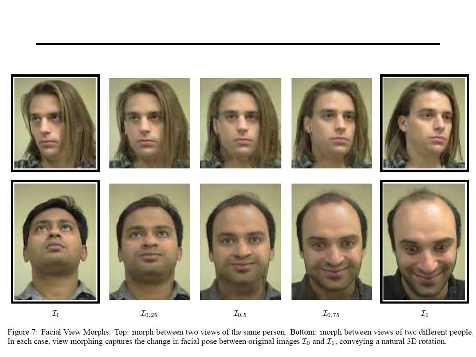
21. Application: View morphing

22. Application: View morphing

23. Problem with morphing
Without rectification

25. Main trick Prewarp with a homography to rectify images
So that the two views are parallel
Because linear interpolation works when views are parallel

26. morph
morph
prewarp
prewarp
output
input
input
homographies

28. Video demo

29. CSE 576 (Spring 2005): Computer Vision
Triangulation
Problem: Given some points in correspondence across two or more images (taken from calibrated cameras), {(uj,vj)}, compute the 3D location X
Richard Szeliski
CSE 576 (Spring 2005): Computer Vision

30. CSE 576 (Spring 2005): Computer Vision
Triangulation
Method I: intersect viewing rays in 3D, minimize:
X is the unknown 3D point
Cj is the optical center of camera j
Vj is the viewing ray for pixel (uj,vj)
sj is unknown distance along Vj
Advantage: geometrically intuitive X Vj Cj
Richard Szeliski
CSE 576 (Spring 2005): Computer Vision

31. CSE 576 (Spring 2005): Computer Vision
Triangulation
Method II: solve linear equations in X
advantage: very simple
Method III: non-linear minimization
advantage: most accurate (image plane error)
Richard Szeliski
CSE 576 (Spring 2005): Computer Vision

32. Structure from motion

33. Structure from motion
Unknown
camera
viewpoints
With what we have discussed so far, we can solve this problem already, in principle.
structure from motion: automatic recovery of camera motion and scene structure from two or more images. It is a self calibration technique and called automatic camera tracking or matchmoving.

34. Applications
For computer vision, multiple-view environment reconstruction, novel view synthesis and autonomous vehicle navigation.
For film production, seamless insertion of CGI into live-action backgrounds

35. Structure from motion SFM pipeline 2D feature geometry optimization
matching
3D estimation
optimization
(bundle adjust)
geometry
fitting
SFM pipeline

36. Structure from motion Step 1: Track Features
Detect good features, Shi & Tomasi, SIFT
Find correspondences between frames
Lucas & Kanade-style motion estimation
window-based correlation
SIFT matching

37. Structure from Motion Step 2: Estimate Motion and Structure
Simplified projection model, e.g., [Tomasi 92]
2 or 3 views at a time [Hartley 00]

38. Structure from Motion Step 3: Refine estimates
“Bundle adjustment” in photogrammetry
Other iterative methods

39. Structure from Motion
Step 4: Recover surfaces (image-based triangulation, silhouettes, stereo…)
Good mesh

40. Example : Photo Tourism

41. Factorization methods

42. Problem statement

43. Other projection models

44. SFM under orthographic projection
matrix
2D image
point
3D scene
point
image
offset
Trick
Choose scene origin to be centroid of 3D points
Choose image origins to be centroid of 2D points
Allows us to drop the camera translation:

45. factorization (Tomasi & Kanade)
projection of n features in one image:
projection of n features in m images
W measurement
M motion
S shape
Key Observation: rank(W) <= 3