1. Non-life insurance mathematics
Nils F. Haavardsson, University of Oslo and DNB Skadeforsikring

2. Repetition claim size The concept Non parametric modelling
Scale families of distributions
Fitting a scale family
Shifted distributions
Skewness
Non parametric estimation
Parametric estimation: the log normal family
Parametric estimation: the gamma family
Parametric estimation: fitting the gamma

3. Claim severity modelling is about describing the variation in claim size
The concept
The graph below shows how claim size varies for fire claims for houses
The graph shows data up to the 88th percentile
How does claim size vary?
How can this variation be modelled?
Truncation is necessary (large claims are rare and disturb the picture)
0-claims can occur (because of deductibles)
Two approaches to claim size modelling – non-parametric and parametric

4. Non-parametric modelling can be useful
Claim size modelling can be non-parametric where each claim zi of the past is assigned a probability 1/n of re-appearing in the future
A new claim is then envisaged as a random variable for which
This is an entirely proper probability distribution
It is known as the empirical distribution and will be useful in Section 9.5.

5. Non-parametric modelling can be useful
Scale families of distributions
All sensible parametric models for claim size are of the form
and Z0 is a standardized random variable corresponding to
The large the scale parameter, the more spread out the distribution

6. Fitting a scale family Models for scale families satisfy
where are the distribution functions of Z and Z0.
Differentiating with respect to z yields the family of density functions
The standard way of fitting such models is through likelihood estimation. If z1,…,zn are the historical claims, the criterion becomes
which is to be maximized with respect to and other parameters.
A useful extension covers situations with censoring.

7. Fitting a scale family Full value insurance:
The insurance company is liable that the object at all times is insured at its true value
First loss insurance
The object is insured up to a pre-specified sum.
The insurance company will cover the claim if the claim size does not exceed the pre-specified sum
The chance of a claim Z exceeding b is , and for nb such events with lower bounds b1,…,bnb the analogous joint probability becomes
Take the logarithm of this product and add it to the log likelihood of the fully observed claims z1,…,zn. The criterion then becomes
complete information
(for objects fully insured)
censoring to the right
(for first loss insured)

8. Shifted distributions
The distribution of a claim may start at some treshold b instead of the origin.
Obvious examples are deductibles and re-insurance contracts.
Models can be constructed by adding b to variables starting at the origin; i.e where Z0 is a standardized variable as before. Now
Example:
Re-insurance company will pay if claim exceeds NOK
The payout of the insurance company
Currency rate for example NOK per EURO, for example 8 NOK per EURO
Total claim amount

9. Skewness as simple description of shape
A major issue with claim size modelling is asymmetry and the right tail of the distribution. A simple summary is the coefficient of skewness
Negative skewness
Positive skewness
Negative skewness: the left tail is longer; the mass of the distribution
Is concentrated on the right of the figure. It has relatively few low values
Positive skewness: the right tail is longer; the mass of the distribution
Is concentrated on the left of the figure. It has relatively few high values

10. Non-parametric estimation
The random variable that attaches probabilities 1/n to all claims zi of the past is a possible model for future claims.
Expectation, standard deviation, skewness and percentiles are all closely related to the ordinary sample versions. For example
Furthermore,
Third order moment and skewness becomes

11. Parametric estimation: the log normal family
A convenient definition of the log-normal model in the present context is
as where
Mean, standard deviation and skewness are
see section 2.4.
Parameter estimation is usually carried out by noting that logarithms are Gaussian. Thus
and when the original log-normal observations z1,…,zn are transformed to Gaussian ones through y1=log(z1),…,yn=log(zn) with sample mean and variance , the estimates of become

12. Parametric estimation: the gamma family
The Gamma family is an important family for which the density function is
It was defined in Section 2.5 as is the standard Gamma with mean one and shape alpha. The density of the standard Gamma simplifies to
Mean, standard deviation and skewness are
and there is a convolution property. Suppose G1,…,Gn are independent with
. Then

13. Parametric estimation: fitting the gamma
The Gamma family
The Gamma family is an important family for which the density function is
It was defined in Section 2.5 as is the standard Gamma with mean one and shape alpha. The density of the standard Gamma simplifies to

14. Parametric estimation: fitting the gamma
The Gamma family

15. Example: car insurance
Non parametric
Log-normal, Gamma
The Pareto
Extreme value
Searching
Hull coverage (i.e., damages on own vehicle in a collision or other sudden and unforeseen damage)
Time period for parameter estimation: 2 years
Covariates:
Car age
Region of car owner
Tariff class
Bonus of insured vehicle
Gamma without zero claims the best model

16. QQ plot Gamma model without zero claims
Non parametric
Log-normal, Gamma
The Pareto
Extreme value
Searching

17. Non parametric
Log-normal, Gamma
The Pareto
Extreme value
Searching

18. Non parametric
Log-normal, Gamma
The Pareto
Extreme value
Searching

19. Non parametric
Log-normal, Gamma
The Pareto
Extreme value
Searching

20. Non parametric
Log-normal, Gamma
The Pareto
Extreme value
Searching

21. Overview

22. The ultimate goal for calculating the pure premium is pricing
Pure premium = Claim frequency x claim severity
Parametric and non parametric modelling (section 9.2 EB)
The log-normal and Gamma families (section 9.3 EB)
The Pareto families (section 9.4 EB)
Extreme value methods (section 9.5 EB)
Searching for the model (section 9.6 EB)

23. The Pareto distribution
Non parametric
Log-normal, Gamma
The Pareto
Extreme value
Searching
The Pareto distributions, introduced in Section 2.5, are among the most heavy-tailed of all models in practical use and potentially a conservative choice when evaluating risk. Density and distribution functions are
Simulation can be done using Algorithm 2.13:
Input alpha and beta
Generate U~Uniform
Return X = beta(U^^(-(1/alpha))-1)
Pareto models are so heavy-tailed that even the mean may fail to exist (that’s why another parameter beta must be used to represent scale). Formulae for expectation, standard deviation and skewness are
valid for alpha>1, alpha>2 and alpha >3 respectively.

24. The Pareto distribution
Non parametric
Log-normal, Gamma
The Pareto
Extreme value
Searching
The median is given by
The exponential distribution appears in the limit when the ratio is kept fixed and
There is in this sense overlap between the Pareto and the Gamma families.
The exponential distribution is a heavy-tailed Gamma and the most light-tailed Pareto and it is common to regard it as a member of both families
Likelihood estimation
The Pareto model was used as illustration in Section 7.3, and likelihood estimation was developed there
Censored information is now added. Suppose observations are in two groups, either the ordinary, fully observed claims z1,..,zn or those only to known to have exceeded certain thresholds b1,..,bn but not by how much.
The log likelihood function for the first group is as in Section 7.3

25. The Pareto distribution
Non parametric
Log-normal, Gamma
The Pareto
Extreme value
Searching
whereas the censored part adds contribution from knowing that Zi>bi.
The probability is
and the full likelihood becomes
Complete information
Censoring to the right
This is to be maximised with respect to , a numerical problem very much the same as in Section 7.3.

26. Over-threshold under Pareto
Non parametric
Log-normal, Gamma
The Pareto
Extreme value
Searching
One of the most important properties of the Pareto family is the behaviour at the extreme right tail. The issue is defined by the over-threshold model which is the distribution of Zb=Z-b given Z>b. Its density function is
The over-threshold density becomes Pareto:
Pareto density function
The shape alpha is the same as before, but the parameter of scale has now changed to
Over-threshold distributions preserve the Pareto model and its shape.
The mean is given by (alpha must exceed 1)

27. The extended Pareto family
Non parametric
Log-normal, Gamma
The Pareto
Extreme value
Searching
Add the numerator to the Pareto density function, and it reads
which defines the extended Pareto model.
Shape is now defined by two parameters , and this creates useful flexibility.
The density function is either decreasing over the positive real line ( if theta <= 1) or has a single maximum (if theta >1). Mean and standard deviation are
Pareto density function
which are valid when alpha > 1 and alpha>2 respectively whereas skewness is
provided alpha > 3. These results verified in Section 9.7 reduce to those for the ordinary Pareto distribution when theta=1.

28. Sampling the extended Pareto family
Non parametric
Log-normal, Gamma
The Pareto
Extreme value
Searching
An extended Pareto variable with parameters can be written
Here G1 and G2 are two independent Gamma variables with mean one.
The representation which is provided in Section 9.7 implies that 1/Z is extended Pareto distributed as well and leads to the following algorithm:
Algorithm 9.1 The extended Pareto sampler
Input and
Draw G1 ~ Gamma(theta)
Draw G2 ~ Gamma(alpha)
Return Z <- etta G1/G2

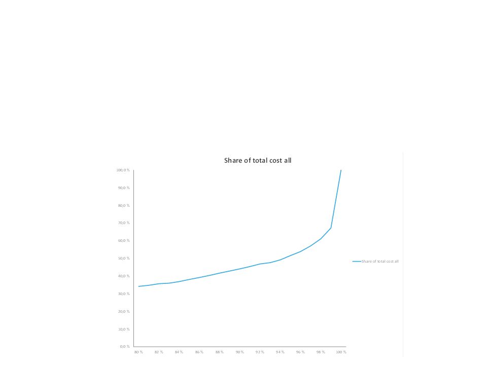
29. Extreme value methods
Non parametric
Log-normal, Gamma
The Pareto
Extreme value
Searching
Large claims play a special role because of their importance financially
The share of large claims is the most important driver for profitability volatility
«The larger claim the greater is the degree of randomness»
But experience is often limited
How should such situations be tackled?
Theory
Pareto distributions are preserved over thresholds
If Z is continuous and unbounded and b is some threshold, then Z-b given Z>b will be Pareto as b grows to infinity!!
…..Ok….
How do we use this?
How large does b has to be?

30. Extreme value methods
Non parametric
Log-normal, Gamma
The Pareto
Extreme value
Searching
Our target is Zb=Z-b given Z>b. Consider its tail distribution function
and let where is a scale parameter depending on b. We are assuming that Z>b, and Yb is then positive with tail distribution The general result says that there exists a parameter alpha (not depending on b and possibly infinite) and some sequence betab such that
The limit is the tail distribution of the Pareto model which shows that Zb becomes Both the shape alpha and the scale parameter betab depend on the original model but only the latter varies with b.

31. Extreme value methods
Non parametric
Log-normal, Gamma
The Pareto
Extreme value
Searching
The decay rate can be determined from historical data
One possibility is to select observations exceeding some threshold, impose the Pareto distribution and use likelihood estimation as explained in Section 9.4. We will revert to this
An alternative often referred to in the literature of extreme value is the Hill estimate
Start by sorting the data in ascending order and take
Here p is some small, user-selected number.
The method is non-parametric (no model is assumed)
We may want to use as an estimate of in a Pareto distribution imposed over the threshold and would then need an estimate of the scale parameter
A practical choice is then

32. The entire distribution through mixtures
Non parametric
Log-normal, Gamma
The Pareto
Extreme value
Searching
Assume some large claim threshold b is selected
Then there are many values in the small and medium range below and up to b and few above b
How to select b?
One way: choose some small probability p and let n1 = integer(n(1-p)) and let b=z(n1))
Another way: study the percentiles
Modelling may be divided into separate parts defined by the threshold b
Modelling in the central region: non-parametric (empirical distribution) or some selected distribution (i.e., log-normal gamma etc)
Modelling in the extreme right tail:
The result due to Pickands suggests a Pareto distribution, provided b is large enough
But is b large enough??
Other distributions may perform better, more about this in Section 9.6.
Central
Region
(plenty of data)
Extreme
right tail
(data is scarce)

33. Non parametric
Log-normal, Gamma
The Pareto
Extreme value
Searching

34. Non parametric
Log-normal, Gamma
The Pareto
Extreme value
Searching

35. Non parametric
Log-normal, Gamma
The Pareto
Extreme value
Searching

36. Non parametric
Log-normal, Gamma
The Pareto
Extreme value
Searching

37. Non parametric
Log-normal, Gamma
The Pareto
Extreme value
Searching

40. Non parametric
Log-normal, Gamma
The Pareto
Extreme value
Searching

41. Non parametric
Log-normal, Gamma
The Pareto
Extreme value
Searching

42. Non parametric
Log-normal, Gamma
The Pareto
Extreme value
Searching

43. Non parametric
Log-normal, Gamma
The Pareto
Extreme value
Searching

44. Non parametric
Log-normal, Gamma
The Pareto
Extreme value
Searching

45. Searching for the model
Non parametric
Log-normal, Gamma
The Pareto
Extreme value
Searching
How is the final model for claim size selected?
Traditional tools: QQ plots and criterion comparisons
Transformations may also be used (see Erik Bølviken’s material)

46. Non parametric
Log-normal, Gamma
The Pareto
Extreme value
Searching

47. Non parametric
Log-normal, Gamma
The Pareto
Extreme value
Searching

48. Non parametric
Log-normal, Gamma
The Pareto
Extreme value
Searching

49. Non parametric
Log-normal, Gamma
The Pareto
Extreme value
Searching

50. Non parametric
Log-normal, Gamma
The Pareto
Extreme value
Searching

51. Non parametric
Log-normal, Gamma
The Pareto
Extreme value
Searching

52. Non parametric
Log-normal, Gamma
The Pareto
Extreme value
Searching

53. Non parametric
Log-normal, Gamma
The Pareto
Extreme value
Searching

54. Non parametric
Log-normal, Gamma
The Pareto
Extreme value
Searching

55. Non parametric
Log-normal, Gamma
The Pareto
Extreme value
Searching

56. Non parametric
Log-normal, Gamma
The Pareto
Extreme value
Searching

57. Non parametric
Log-normal, Gamma
The Pareto
Extreme value
Searching

58. Searching for the model
Non parametric
Log-normal, Gamma
The Pareto
Extreme value
Searching
Can we do better?
Does it exist a more generic class of distribution with these distributions as special cases?
Does this generic class of distributions outperform the selected model in the two examples (fire above 90th percentile and fire above 95th percentile)?