1. Empirical Methods for Microeconomic Applications University of Lugano, Switzerland May 27-31, 2013 William Greene Department of Economics Stern School of Business

2. 1C. Extensions of Binary Choice Models

3. Agenda for 1C Endogenous RHS Variables Sample Selection Dynamic Binary Choice Model Bivariate Binary Choice Simultaneous Equations Ordered Choices Ordered Choice Model Application to BHPS

4. Endogeneity

5. Endogenous RHS Variable U* = β’x + θh + ε y = 1[U* > 0] E[ε|h] ≠ 0 (h is endogenous) Case 1: h is continuous Case 2: h is binary, e.g., a treatment effect Approaches Parametric: Maximum Likelihood Semiparametric (not developed here):  GMM  Various approaches for case 2

6. Endogenous Continuous Variable U* = β’x + θh + ε y = 1[U* > 0]  h = α’z + u E[ε|h] ≠ 0  Cov[u, ε] ≠ 0 Additional Assumptions: (u,ε) ~ N[(0,0),(σ u 2, ρσ u, 1)] z = a valid set of exogenous variables, uncorrelated with (u, ε) Correlation = ρ. This is the source of the endogeneity

7. Endogenous Income in Health 0 = Not Healthy 1 = Healthy Healthy = 0 or 1 Age, Married, Kids, Gender, Income Determinants of Income (observed and unobserved) also determine health satisfaction. Income responds to Age, Age 2, Educ, Married, Kids, Gender

8. Estimation by ML (Control Function)

9. Two Approaches to ML

10. FIML Estimates ---------------------------------------------------------------------- Probit with Endogenous RHS Variable Dependent variable HEALTHY Log likelihood function -6464.60772 --------+------------------------------------------------------------- Variable| Coefficient Standard Error b/St.Er. P[|Z|>z] Mean of X --------+------------------------------------------------------------- |Coefficients in Probit Equation for HEALTHY Constant| 1.21760***.06359 19.149.0000 AGE| -.02426***.00081 -29.864.0000 43.5257 MARRIED| -.02599.02329 -1.116.2644.75862 HHKIDS|.06932***.01890 3.668.0002.40273 FEMALE| -.14180***.01583 -8.959.0000.47877 INCOME|.53778***.14473 3.716.0002.35208 |Coefficients in Linear Regression for INCOME Constant| -.36099***.01704 -21.180.0000 AGE|.02159***.00083 26.062.0000 43.5257 AGESQ| -.00025***.944134D-05 -26.569.0000 2022.86 EDUC|.02064***.00039 52.729.0000 11.3206 MARRIED|.07783***.00259 30.080.0000.75862 HHKIDS| -.03564***.00232 -15.332.0000.40273 FEMALE|.00413**.00203 2.033.0420.47877 |Standard Deviation of Regression Disturbances Sigma(w)|.16445***.00026 644.874.0000 |Correlation Between Probit and Regression Disturbances Rho(e,w)| -.02630.02499 -1.052.2926 --------+-------------------------------------------------------------

11. Partial Effects: Scaled Coefficients

12. Endogenous Binary Variable U* = β’x + θh + ε y = 1[U* > 0] h* = α’z + u h = 1[h* > 0] E[ε|h*] ≠ 0  Cov[u, ε] ≠ 0 Additional Assumptions: (u,ε) ~ N[(0,0),(σ u 2, ρσ u, 1)] z = a valid set of exogenous variables, uncorrelated with (u, ε) Correlation = ρ. This is the source of the endogeneity 

13. Endogenous Binary Variable Doctor = F(age,age 2,income,female,Public)Public = F(age,educ,income,married,kids,female)

14. FIML Estimates ---------------------------------------------------------------------- FIML Estimates of Bivariate Probit Model Dependent variable DOCPUB Log likelihood function -25671.43905 Estimation based on N = 27326, K = 14 --------+------------------------------------------------------------- Variable| Coefficient Standard Error b/St.Er. P[|Z|>z] Mean of X --------+------------------------------------------------------------- |Index equation for DOCTOR Constant|.59049***.14473 4.080.0000 AGE| -.05740***.00601 -9.559.0000 43.5257 AGESQ|.00082***.681660D-04 12.100.0000 2022.86 INCOME|.08883*.05094 1.744.0812.35208 FEMALE|.34583***.01629 21.225.0000.47877 PUBLIC|.43533***.07357 5.917.0000.88571 |Index equation for PUBLIC Constant| 3.55054***.07446 47.681.0000 AGE|.00067.00115.581.5612 43.5257 EDUC| -.16839***.00416 -40.499.0000 11.3206 INCOME| -.98656***.05171 -19.077.0000.35208 MARRIED| -.00985.02922 -.337.7361.75862 HHKIDS| -.08095***.02510 -3.225.0013.40273 FEMALE|.12139***.02231 5.442.0000.47877 |Disturbance correlation RHO(1,2)| -.17280***.04074 -4.241.0000 --------+-------------------------------------------------------------

15. Partial Effects

16. Identification Issues Exclusions are not needed for estimation Identification is, in principle, by “functional form” Researchers usually have a variable in the treatment equation that is not in the main probit equation “to improve identification” A fully simultaneous model y1 = f(x1,y2), y2 = f(x2,y1) Not identified even with exclusion restrictions (Model is “incoherent”)

17. Selection

18. A Sample Selection Model U* = β’x + ε y = 1[U* > 0] h* = α’z + u h = 1[h* > 0] E[ε|h] ≠ 0  Cov[u, ε] ≠ 0 (y,x) are observed only when h = 1 Additional Assumptions: (u,ε) ~ N[(0,0),(σ u 2, ρσ u, 1)] z = a valid set of exogenous variables, uncorrelated with (u,ε) Correlation = ρ. This is the source of the “selectivity:

19. Application: Doctor,Public 3 Groups of observations: (Public=0), (Doctor=0|Public=1), (Doctor=1|Public=1)

20. Sample Selection Doctor = F(age,age 2,income,female,Public=1) Public = F(age,educ,income,married,kids,female)

21. Sample Selection Model: Estimation

22. ML Estimates ---------------------------------------------------------------------- FIML Estimates of Bivariate Probit Model Dependent variable DOCPUB Log likelihood function -23581.80697 Estimation based on N = 27326, K = 13 Selection model based on PUBLIC Means for vars. 1- 5 are after selection. --------+------------------------------------------------------------- Variable| Coefficient Standard Error b/St.Er. P[|Z|>z] Mean of X --------+------------------------------------------------------------- |Index equation for DOCTOR Constant| 1.09027***.13112 8.315.0000 AGE| -.06030***.00633 -9.532.0000 43.6996 AGESQ|.00086***.718153D-04 11.967.0000 2041.87 INCOME|.07820.05779 1.353.1760.33976 FEMALE|.34357***.01756 19.561.0000.49329 |Index equation for PUBLIC Constant| 3.54736***.07456 47.580.0000 AGE|.00080.00116.690.4899 43.5257 EDUC| -.16832***.00416 -40.490.0000 11.3206 INCOME| -.98747***.05162 -19.128.0000.35208 MARRIED| -.01508.02934 -.514.6072.75862 HHKIDS| -.07777***.02514 -3.093.0020.40273 FEMALE|.12154***.02231 5.447.0000.47877 |Disturbance correlation RHO(1,2)| -.19303***.06763 -2.854.0043 --------+-------------------------------------------------------------

23. Estimation Issues This is a sample selection model applied to a nonlinear model There is no lambda Estimated by FIML, not two step least squares Estimator is a type of BIVARIATE PROBIT MODEL The model is identified without exclusions (again)

24. A Dynamic Model

25. Dynamic Models

26. Dynamic Probit Model: A Standard Approach

27. Simplified Dynamic Model

28. A Dynamic Model for Public Insurance

29. Dynamic Common Effects Model

30. Bivariate Model

31. Gross Relation Between Two Binary Variables Cross Tabulation Suggests Presence or Absence of a Bivariate Relationship +-----------------------------------------------------------------+ |Cross Tabulation | |Row variable is DOCTOR (Out of range 0-49: 0) | |Number of Rows = 2 (DOCTOR = 0 to 1) | |Col variable is HOSPITAL (Out of range 0-49: 0) | |Number of Cols = 2 (HOSPITAL = 0 to 1) | +-----------------------------------------------------------------+ | HOSPITAL | +--------+--------------+------+ | | DOCTOR| 0 1| Total| | +--------+--------------+------+ | | 0| 9715 420| 10135| | | 1| 15216 1975| 17191| | +--------+--------------+------+ | | Total| 24931 2395| 27326| | +-----------------------------------------------------------------+

32. Tetrachoric Correlation

33. Log Likelihood Function for Tetrachoric Correlation

34. Estimation +---------------------------------------------+ | FIML Estimates of Bivariate Probit Model | | Maximum Likelihood Estimates | | Dependent variable DOCHOS | | Weighting variable None | | Number of observations 27326 | | Log likelihood function -25898.27 | | Number of parameters 3 | +---------------------------------------------+ +---------+--------------+----------------+--------+---------+ |Variable | Coefficient | Standard Error |b/St.Er.|P[|Z|>z] | +---------+--------------+----------------+--------+---------+ Index equation for DOCTOR Constant.32949128.00773326 42.607.0000 Index equation for HOSPITAL Constant -1.35539755.01074410 -126.153.0000 Tetrachoric Correlation between DOCTOR and HOSPITAL RHO(1,2).31105965.01357302 22.918.0000

35. A Bivariate Probit Model Two Equation Probit Model No bivariate logit – there is no reasonable bivariate counterpart Why fit the two equation model? Analogy to SUR model: Efficient Make tetrachoric correlation conditional on covariates – i.e., residual correlation

36. Bivariate Probit Model

37. Estimation of the Bivariate Probit Model

38. Parameter Estimates ---------------------------------------------------------------------- FIML Estimates of Bivariate Probit Model for DOCTOR and HOSPITAL Dependent variable DOCHOS Log likelihood function -25323.63074 Estimation based on N = 27326, K = 12 --------+------------------------------------------------------------- Variable| Coefficient Standard Error b/St.Er. P[|Z|>z] Mean of X --------+------------------------------------------------------------- |Index equation for DOCTOR Constant| -.20664***.05832 -3.543.0004 AGE|.01402***.00074 18.948.0000 43.5257 FEMALE|.32453***.01733 18.722.0000.47877 EDUC| -.01438***.00342 -4.209.0000 11.3206 MARRIED|.00224.01856.121.9040.75862 WORKING| -.08356***.01891 -4.419.0000.67705 |Index equation for HOSPITAL Constant| -1.62738***.05430 -29.972.0000 AGE|.00509***.00100 5.075.0000 43.5257 FEMALE|.12143***.02153 5.641.0000.47877 HHNINC| -.03147.05452 -.577.5638.35208 HHKIDS| -.00505.02387 -.212.8323.40273 |Disturbance correlation (Conditional tetrachoric correlation) RHO(1,2)|.29611***.01393 21.253.0000 ---------------------------------------------------------------------- | Tetrachoric Correlation between DOCTOR and HOSPITAL RHO(1,2)|.31106.01357 22.918.0000 --------+-------------------------------------------------------------

39. Marginal Effects What are the marginal effects Effect of what on what? Two equation model, what is the conditional mean? Possible margins? Derivatives of joint probability = Φ 2 (β 1 ’x i1, β 2 ’x i2,ρ) Partials of E[y ij |x ij ] =Φ(β j ’x ij ) (Univariate probability) Partials of E[y i1 |x i1,x i2,y i2 =1] = P(y i1,y i2 =1)/Prob[y i2 =1] Note marginal effects involve both sets of regressors. If there are common variables, there are two effects in the derivative that are added.

40. Bivariate Probit Conditional Means

41. Direct Effects Derivatives of E[y 1 |x 1,x 2,y 2 =1] wrt x 1 +-------------------------------------------+ | Partial derivatives of E[y1|y2=1] with | | respect to the vector of characteristics. | | They are computed at the means of the Xs. | | Effect shown is total of 4 parts above. | | Estimate of E[y1|y2=1] =.819898 | | Observations used for means are All Obs. | | These are the direct marginal effects. | +-------------------------------------------+ +---------+--------------+----------------+--------+---------+----------+ |Variable | Coefficient | Standard Error |b/St.Er.|P[|Z|>z] | Mean of X| +---------+--------------+----------------+--------+---------+----------+ AGE.00382760.00022088 17.329.0000 43.5256898 FEMALE.08857260.00519658 17.044.0000.47877479 EDUC -.00392413.00093911 -4.179.0000 11.3206310 MARRIED.00061108.00506488.121.9040.75861817 WORKING -.02280671.00518908 -4.395.0000.67704750 HHNINC.000000......(Fixed Parameter)........35208362 HHKIDS.000000......(Fixed Parameter)........40273000

42. Indirect Effects Derivatives of E[y 1 |x 1,x 2,y 2 =1] wrt x 2 +-------------------------------------------+ | Partial derivatives of E[y1|y2=1] with | | respect to the vector of characteristics. | | They are computed at the means of the Xs. | | Effect shown is total of 4 parts above. | | Estimate of E[y1|y2=1] =.819898 | | Observations used for means are All Obs. | | These are the indirect marginal effects. | +-------------------------------------------+ +---------+--------------+----------------+--------+---------+----------+ |Variable | Coefficient | Standard Error |b/St.Er.|P[|Z|>z] | Mean of X| +---------+--------------+----------------+--------+---------+----------+ AGE -.00035034.697563D-04 -5.022.0000 43.5256898 FEMALE -.00835397.00150062 -5.567.0000.47877479 EDUC.000000......(Fixed Parameter)....... 11.3206310 MARRIED.000000......(Fixed Parameter)........75861817 WORKING.000000......(Fixed Parameter)........67704750 HHNINC.00216510.00374879.578.5636.35208362 HHKIDS.00034768.00164160.212.8323.40273000

43. Marginal Effects: Total Effects Sum of Two Derivative Vectors +-------------------------------------------+ | Partial derivatives of E[y1|y2=1] with | | respect to the vector of characteristics. | | They are computed at the means of the Xs. | | Effect shown is total of 4 parts above. | | Estimate of E[y1|y2=1] =.819898 | | Observations used for means are All Obs. | | Total effects reported = direct+indirect. | +-------------------------------------------+ +---------+--------------+----------------+--------+---------+----------+ |Variable | Coefficient | Standard Error |b/St.Er.|P[|Z|>z] | Mean of X| +---------+--------------+----------------+--------+---------+----------+ AGE.00347726.00022941 15.157.0000 43.5256898 FEMALE.08021863.00535648 14.976.0000.47877479 EDUC -.00392413.00093911 -4.179.0000 11.3206310 MARRIED.00061108.00506488.121.9040.75861817 WORKING -.02280671.00518908 -4.395.0000.67704750 HHNINC.00216510.00374879.578.5636.35208362 HHKIDS.00034768.00164160.212.8323.40273000

44. Marginal Effects: Dummy Variables Using Differences of Probabilities +-----------------------------------------------------------+ | Analysis of dummy variables in the model. The effects are | | computed using E[y1|y2=1,d=1] - E[y1|y2=1,d=0] where d is | | the variable. Variances use the delta method. The effect | | accounts for all appearances of the variable in the model.| +-----------------------------------------------------------+ |Variable Effect Standard error t ratio (deriv) | +-----------------------------------------------------------+ FEMALE.079694.005290 15.065 (.080219) MARRIED.000611.005070.121 (.000511) WORKING -.022485.005044 -4.457 (-.022807) HHKIDS.000348.001641.212 (.000348) Computed using difference of probabilities Computed using scaled coefficients

45. Simultaneous Equations

46. A Simultaneous Equations Model bivariate probit;lhs=doctor,hospital ;rh1=one,age,educ,married,female,hospital ;rh2=one,age,educ,married,female,doctor$ Error 809: Fully simultaneous BVP model is not identified

47. Fully Simultaneous ‘Model’ (Obtained by bypassing internal control) ---------------------------------------------------------------------- FIML Estimates of Bivariate Probit Model Dependent variable DOCHOS Log likelihood function -20318.69455 --------+------------------------------------------------------------- Variable| Coefficient Standard Error b/St.Er. P[|Z|>z] Mean of X --------+------------------------------------------------------------- |Index equation for DOCTOR Constant| -.46741***.06726 -6.949.0000 AGE|.01124***.00084 13.353.0000 43.5257 FEMALE|.27070***.01961 13.807.0000.47877 EDUC| -.00025.00376 -.067.9463 11.3206 MARRIED| -.00212.02114 -.100.9201.75862 WORKING| -.00362.02212 -.164.8701.67705 HOSPITAL| 2.04295***.30031 6.803.0000.08765 |Index equation for HOSPITAL Constant| -1.58437***.08367 -18.936.0000 AGE| -.01115***.00165 -6.755.0000 43.5257 FEMALE| -.26881***.03966 -6.778.0000.47877 HHNINC|.00421.08006.053.9581.35208 HHKIDS| -.00050.03559 -.014.9888.40273 DOCTOR| 2.04479***.09133 22.389.0000.62911 |Disturbance correlation RHO(1,2)| -.99996***.00048 ********.0000 --------+-------------------------------------------------------------

48. A Latent Simultaneous Equations Model

49. A Recursive Simultaneous Equations Model

54. Ordered Choices

55. Ordered Discrete Outcomes E.g.: Taste test, credit rating, course grade, preference scale Underlying random preferences: Existence of an underlying continuous preference scale Mapping to observed choices Strength of preferences is reflected in the discrete outcome Censoring and discrete measurement The nature of ordered data

56. Bond Ratings

57. Health Satisfaction (HSAT) Self administered survey: Health Satisfaction (0 – 10) Continuous Preference Scale

58. Modeling Ordered Choices Random Utility (allowing a panel data setting) U it =  +  ’x it +  it = a it +  it Observe outcome j if utility is in region j Probability of outcome = probability of cell Pr[Y it =j] = Prob[Y it < j] - Prob[Y it < j-1] = F(  j – a it ) - F(  j-1 – a it )

59. Ordered Probability Model

60. Combined Outcomes for Health Satisfaction

61. Probabilities for Ordered Choices

62. μ 1 =1.1479 μ 2 =2.5478 μ 3 =3.0564

63. Coefficients

64. Effects of 8 More Years of Education

65. An Ordered Probability Model for Health Satisfaction +---------------------------------------------+ | Ordered Probability Model | | Dependent variable HSAT | | Number of observations 27326 | | Underlying probabilities based on Normal | | Cell frequencies for outcomes | | Y Count Freq Y Count Freq Y Count Freq | | 0 447.016 1 255.009 2 642.023 | | 3 1173.042 4 1390.050 5 4233.154 | | 6 2530.092 7 4231.154 8 6172.225 | | 9 3061.112 10 3192.116 | +---------------------------------------------+ +---------+--------------+----------------+--------+---------+----------+ |Variable | Coefficient | Standard Error |b/St.Er.|P[|Z|>z] | Mean of X| +---------+--------------+----------------+--------+---------+----------+ Index function for probability Constant 2.61335825.04658496 56.099.0000 FEMALE -.05840486.01259442 -4.637.0000.47877479 EDUC.03390552.00284332 11.925.0000 11.3206310 AGE -.01997327.00059487 -33.576.0000 43.5256898 HHNINC.25914964.03631951 7.135.0000.35208362 HHKIDS.06314906.01350176 4.677.0000.40273000 Threshold parameters for index Mu(1).19352076.01002714 19.300.0000 Mu(2).49955053.01087525 45.935.0000 Mu(3).83593441.00990420 84.402.0000 Mu(4) 1.10524187.00908506 121.655.0000 Mu(5) 1.66256620.00801113 207.532.0000 Mu(6) 1.92729096.00774122 248.965.0000 Mu(7) 2.33879408.00777041 300.987.0000 Mu(8) 2.99432165.00851090 351.822.0000 Mu(9) 3.45366015.01017554 339.408.0000

66. Ordered Probit Partial Effects Partial effects at means of the data Average Partial Effect of HHNINC

67. Predictions of the Model:Kids +----------------------------------------------+ |Variable Mean Std.Dev. Minimum Maximum | +----------------------------------------------+ |Stratum is KIDS = 0.000. Nobs.= 2782.000 | +--------+-------------------------------------+ |P0 |.059586.028182.009561.125545 | |P1 |.268398.063415.106526.374712 | |P2 |.489603.024370.419003.515906 | |P3 |.101163.030157.052589.181065 | |P4 |.081250.041250.028152.237842 | +----------------------------------------------+ |Stratum is KIDS = 1.000. Nobs.= 1701.000 | +--------+-------------------------------------+ |P0 |.036392.013926.010954.105794 | |P1 |.217619.039662.115439.354036 | |P2 |.509830.009048.443130.515906 | |P3 |.125049.019454.061673.176725 | |P4 |.111111.030413.035368.222307 | +----------------------------------------------+ |All 4483 observations in current sample | +--------+-------------------------------------+ |P0 |.050786.026325.009561.125545 | |P1 |.249130.060821.106526.374712 | |P2 |.497278.022269.419003.515906 | |P3 |.110226.029021.052589.181065 | |P4 |.092580.040207.028152.237842 | +----------------------------------------------+ This is a restricted model with outcomes collapsed into 5 cells.

68. Fit Measures There is no single “dependent variable” to explain. There is no sum of squares or other measure of “variation” to explain. Predictions of the model relate to a set of J+1 probabilities, not a single variable. How to explain fit? Based on the underlying regression Based on the likelihood function Based on prediction of the outcome variable

69. Log Likelihood Based Fit Measures

70. Fit Measure Based on Counting Predictions This model always predicts the same cell.

71. A Somewhat Better Fit

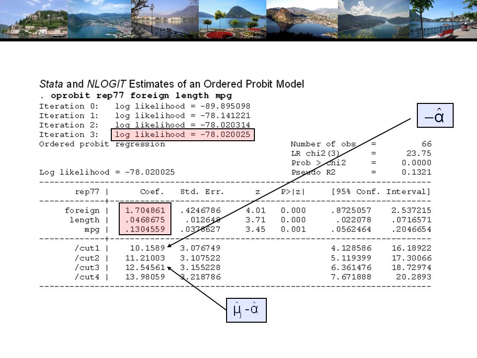
72. Different Normalizations NLOGIT Y = 0,1,…,J, U* = α + β’x + ε One overall constant term, α J-1 “thresholds;” μ -1 = -∞, μ 0 = 0, μ 1,… μ J-1, μ J = + ∞ Stata Y = 1,…,J+1, U* = β’x + ε No overall constant, α=0 J “cutpoints;” μ 0 = -∞, μ 1,… μ J, μ J+1 = + ∞

75. Generalizing the Ordered Probit with Heterogeneous Thresholds

76. Differential Item Functioning People in this country are optimistic – they report this value as ‘very good.’ People in this country are pessimistic – they report this same value as ‘fair’

77. Panel Data Fixed Effects The usual incidental parameters problem Partitioning Prob(y it > j|x it ) produces estimable binomial logit models. (Find a way to combine multiple estimates of the same β. Random Effects Standard application

78. Incidental Parameters Problem Table 9.1 Monte Carlo Analysis of the Bias of the MLE in Fixed Effects Discrete Choice Models (Means of empirical sampling distributions, N = 1,000 individuals, R = 200 replications)

80. Random Effects

81. Dynamic Ordered Probit Model

82. Model for Self Assessed Health British Household Panel Survey (BHPS) Waves 1-8, 1991-1998 Self assessed health on 0,1,2,3,4 scale Sociological and demographic covariates Dynamics – inertia in reporting of top scale Dynamic ordered probit model Balanced panel – analyze dynamics Unbalanced panel – examine attrition

83. Dynamic Ordered Probit Model It would not be appropriate to include h i,t-1 itself in the model as this is a label, not a measure

84. Testing for Attrition Bias Three dummy variables added to full model with unbalanced panel suggest presence of attrition effects.

85. Attrition Model with IP Weights Assumes (1) Prob(attrition|all data) = Prob(attrition|selected variables) (ignorability) (2) Attrition is an ‘absorbing state.’ No reentry. Obviously not true for the GSOEP data above. Can deal with point (2) by isolating a subsample of those present at wave 1 and the monotonically shrinking subsample as the waves progress.

86. Inverse Probability Weighting

87. Estimated Partial Effects by Model

88. Partial Effect for a Category These are 4 dummy variables for state in the previous period. Using first differences, the 0.234 estimated for SAHEX means transition from EXCELLENT in the previous period to GOOD in the previous period, where GOOD is the omitted category. Likewise for the other 3 previous state variables. The margin from ‘POOR’ to ‘GOOD’ was not interesting in the paper. The better margin would have been from EXCELLENT to POOR, which would have (EX,POOR) change from (1,0) to (0,1).